Power Query is this awesome feature built right into Exccel that makes handling data so much easier (even millions of rows and hundreds of columns of data).
It allows you to allows you to perform data management’s Extract, Transform, and Load (ETL) processes with an easy-to-use interface (takes only a few clicks):
- Extract (or Get) data – Power Query lets you pull data from pretty much anywhere and grab just the bits you need.
- Transform – Once you’ve got your data, you can play around with it in the Power Query Editor. Want to remove duplicate records? Delete some columns? Remove errors? No problem!
- Load – When you’re happy with your transformed data, Power Query helps you pop it into your workbook or data model. You can even set up a direct connection, create a PivotTable or PivotChart right away, and refresh the data whenever you need the latest info.
The beauty of Power Query is how it connects to tons of different data sources and lets you shape that data just the way you want it.
Remove columns, change data types, merge tables – whatever you need! Then you can use the results to make awesome charts and reports in Excel.
And the best part? You can refresh everything with a click when your source data changes. No more copying and pasting or manual updates!
Power Query basically takes all that tedious ETL work and makes it super simple – pulling data from different places, cleaning it up just how you like it, and dropping it right into your workbook without all the usual headaches.
Note: In Excel 2010 and 2013, Power Query is available as an installable add-in. You can download it from here: Download Microsoft Power Query for Excel.
Key Benefits of Using Power Query
While there are a lot of benefits of using Power Query, here are some major ones:
- Automate data import and transformation, eliminating repetitive manual tasks.
- Connects to multiple data sources such as Excel, CSV, databases (SQL, MS Access), Sharepoint, web data, and many more.
- Easily remove duplicates, split/merge columns, filter data, and handle missing values without complex formulas.
- Append or merge datasets from multiple files or sources with ease.
- Handle large volumes of data more efficiently.
- Refresh queries to update reports.
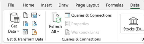
Where to Find Power Query in Excel
You can access Power Query data import wizards and other options from the Data tab’s Get & Transform Data and Queries & Connections groups.
Note: In Excel 2010 and 2013, once installed, the Power Query functionality can be accessed from the Power Query tab on the Ribbon.
Power Query Data Sources
A key benefit of Power Query is its ability to retrieve data from a wide range of sources.
On the Data tab, open the Get Data drop-down on the Get & Transform Data group to view the five categories of data sources from which Power Query can retrieve data.
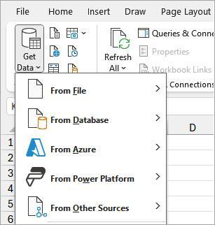
Below is a description of each data source category.
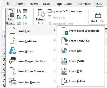
From File
Gets data from an Excel workbook, text file, CSV file, XML file, JSON file, PDF file, or folder.
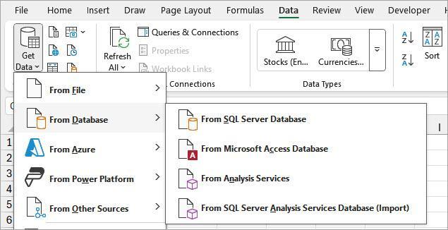
From Database
Extracts data from databases like SQL Server, Microsoft Access, or SQL Server Analysis Services.
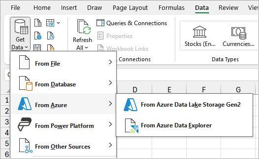
From Azure
Gets data from Microsoft’s Azure Cloud Services.
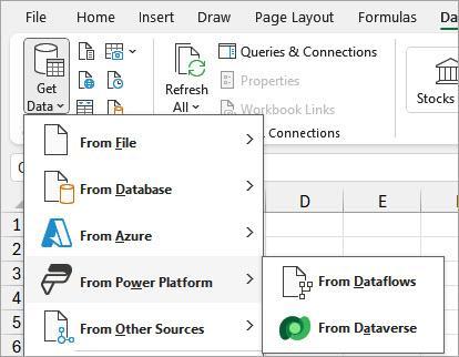
From Power Platform
Pulls data from Power BI and cloud application services like Salesforce and Microsoft Dynamics online.
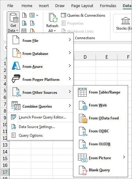
From Other Sources
Pulls data from Excel tables or ranges, websites, ODBC data sources, pictures, and blank queries, which allow you to create custom queries from scratch using Power Query’s M language.
An Example of How to Use Power Query
Let me walk you through a simple example of how to use Power Query.
Suppose you have the historical data of Microsoft Corporation stock prices in a worksheet, as shown below.
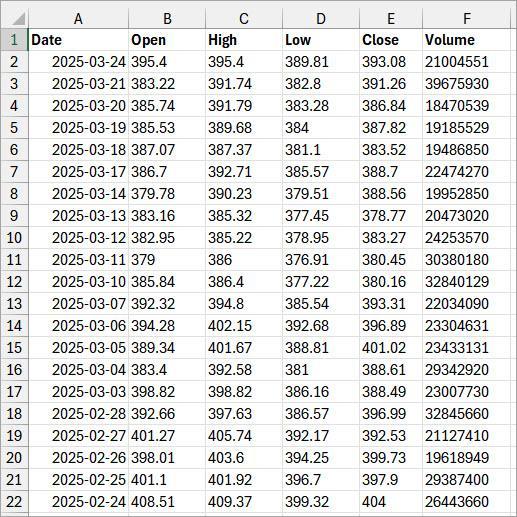
Notice that the Open, High, Low, Close, and Volume data are left-aligned, indicating they are stored as text strings.
You want to load the data onto the Power Query Editor and apply specific actions to clean, shape, and transform it before loading it back onto Excel for analysis.
Here’s how to do it:
Step #1: Extract or Get the Data
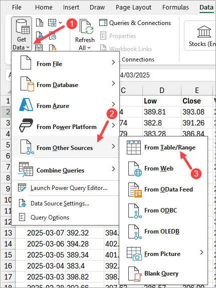
- Select any cell in the dataset.
- Click the Data tab, open the Get Data drop-down list on the Get & Transform group, hover over the From Other Sources option, and click the From Table/Range option on the flyout menu.
The above step opens the Create Table dialog box. The reference to the source data is filled in, and the ‘My table has headers’ checkbox is selected.
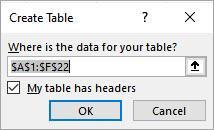
- Click OK on the Create Table dialog box.
The above step converts the base dataset to an Excel table, activates the Power Query Editor window, and displays a preview of the query data in the Data Preview pane.
Notice that the Open, High, Low, Close, and Volume data are now right-aligned, indicating that Power Query has automatically converted them to numeric values. Notice the ‘Changed Type’ applied step in the Applied Steps section of the Query Settings pane.
Note: Refer to the ‘Power Query Editor Interface’ section for a description of each component of the Power Query Editor interface.
Step #2: Transform the Data
To transform or modify the data, you work with each column in the Power Query Editor window, applying the actions yielding the desired data and structure.
Here are the steps to transform the data:
- Click the header of the High column, hold down the CTRL key, and click the headers of the Low and Close columns.
- Right-click the header of one of the selected columns, hover over the Change Type option on the menu, and click the Currency option on the submenu.
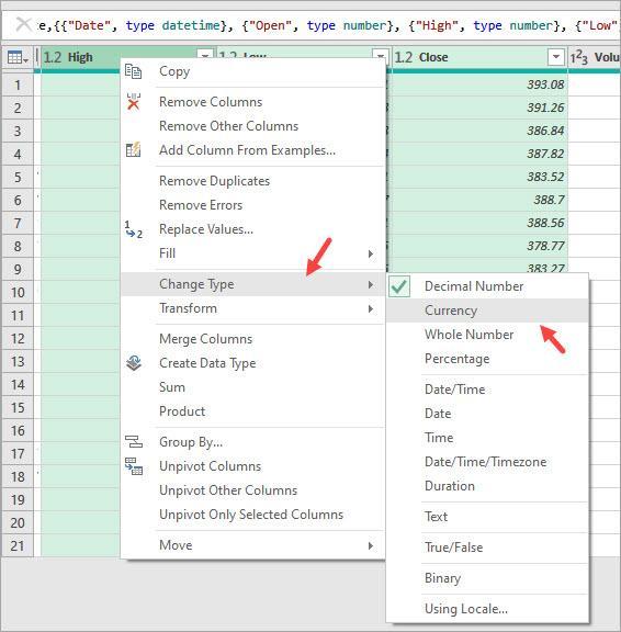
The above step opens the Change Column Type feature, notifying you that the selected columns already have a type conversion (the one that Power Query automatically applied when you loaded the data).
The feature allows you to either replace the existing conversion or preserve it by adding the new conversion as a separate step.
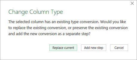
- Click the ‘Add new step’ command button to add the conversion as a separate step.
Notice the dollar sign symbols in the headers of the High, Low, and Close columns, indicating that the data has been converted to ca urrency data type. Also, notice that a new ‘Changed Type1’ step has been added to the Applied Steps section of the Query Settings pane.
- Click the header of the Open column, hold down the CTRL key, and click the header of the Volume column.
- Right-click the header of one of the selected columns and click the Remove Columns option on the shortcut menu.
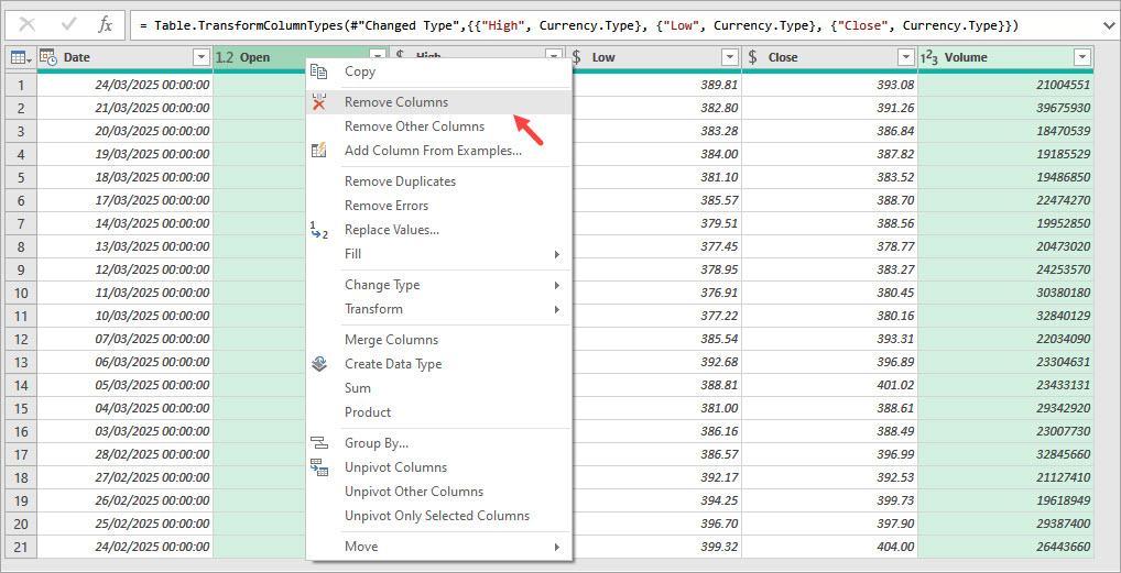
The above step removes the target columns from the query and adds the ‘Removed Columns’ step to the Applied Steps section of the Query Settings pane.
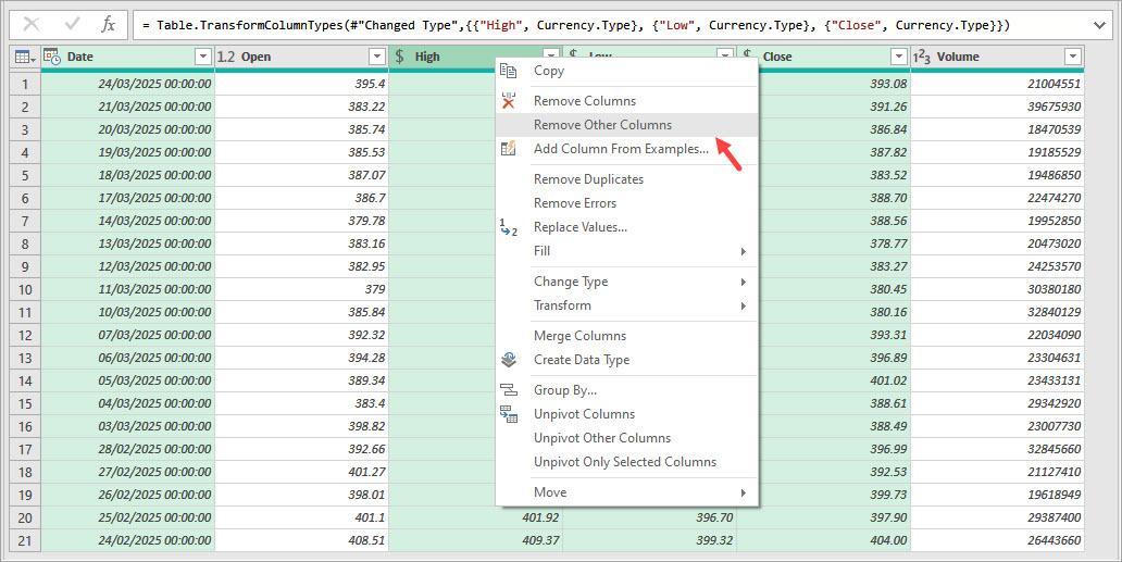
Another way to remove unwanted columns is to select the columns you want to keep and click the Remove Other Columns option on the shortcut menu.
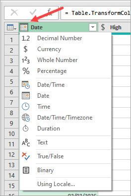
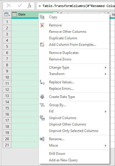
- Right-click the header of the Date column, hover over the Change Type option on the shortcut menu, and click the Date option on the submenu.
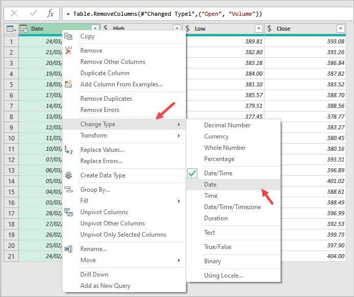
The above step removes the time component from the date values in the Date column and adds the ‘Changed Type2’ step on the Applied Steps box on the Query Settings pane.
- Right-click the header of the Date column and select the Duplicate Column option on the shortcut menu.
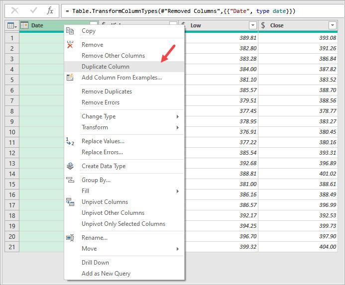
The above step adds a new column, Date – Copy, on the Data Preview pane.
- Right-click the header of the newly added column, select the Rename option on the shortcut menu, and rename the new column ‘Week Of.’
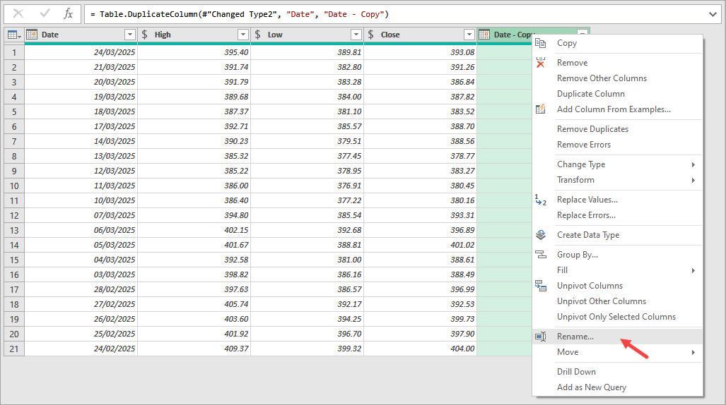
Alternatively, double-click the header of the column and type in the new name.
The above step adds the ‘Renamed Columns’ step to the Applied Steps box on the Query Settings pane.
- Right-click the header of the ‘Week Of’ column, hover over the Transform option on the shortcut menu, hover over the Week option on the submenu, and click the Start of Week option on the last submenu.
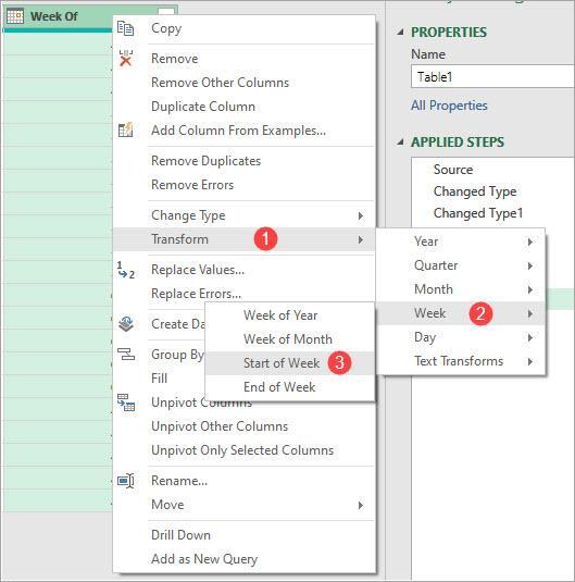
The above step transforms the date values in the column to display the start of the week for the corresponding date in the Date column.
Additionally, it adds the step ‘Calculated Start of the Week’ to the Applied Steps box on the Query Settings pane.
Step #3: Load the Data on a Worksheet
Once you’ve completed transforming the data, use the below steps to output the results to a worksheet.
- Click the Home tab, open the Close & Load drop-down to expose the Close & Load and Close & Load To options.
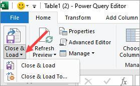
The Close & Load option saves your query and loads the results as an Excel table in a new worksheet in your workbook.
The Close & Load To option opens the Import Data dialog box, allowing you to specify whether to output the results to a particular worksheet as a table, PivotTable report, PivotChart, or add them to the internal data model.
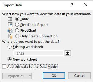
The Import Data dialog box also allows you to save the query as a connection only, meaning you can utilize the query for various in-memory processes without requiring an output of the results.
In this case, I select the ‘New worksheet’ option to output the query results to a new worksheet in the workbook.
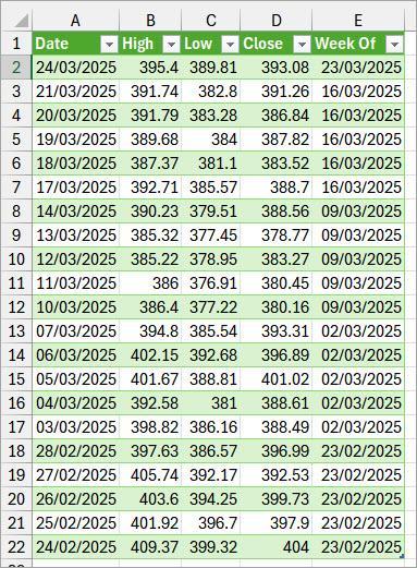
Now, you can appreciate the power of Power Query. With just a few clicks, you’ve transformed the base dataset by keeping only the necessary columns and even added a Week Of column—all without writing a single line of code.
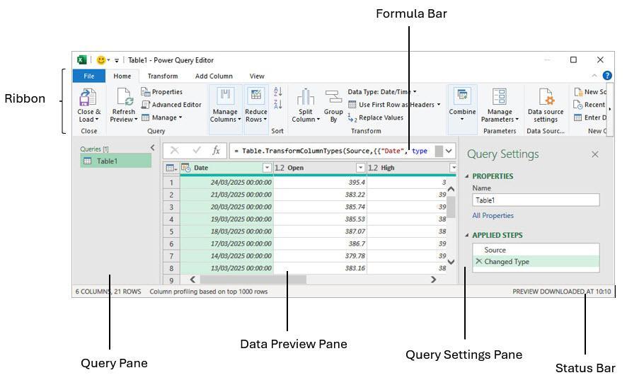
Power Query Editor Interface
The Power Query Editor has the components described below that you can use to clean, shape, and transform your data.
- The Ribbon, consisting of:
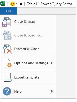
- File tab – Use options on this tab to load data, close the Power Query Editor, access Power Query Help contents, and so on.
- Home tab – Use options on this tab to perform actions such as remove columns and rows, split columns, merge queries, append queries, update the query preview with the latest data, and load the transformed data into Excel.
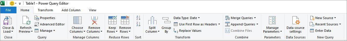
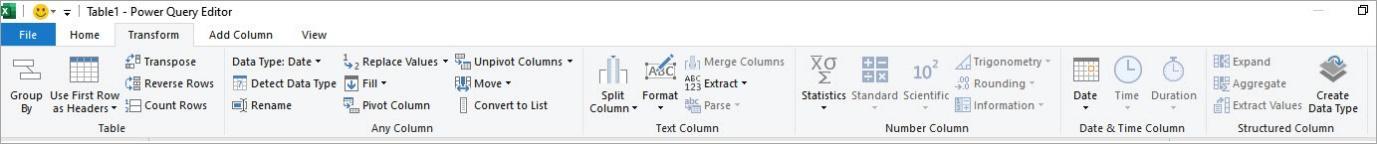
- Transform tab – Use options on this tab to perform various data transformations, such as convert a column’s data type, turn row values into column headers, replace specific values in a column, extract parts of a text value, and split a column into multiple columns.
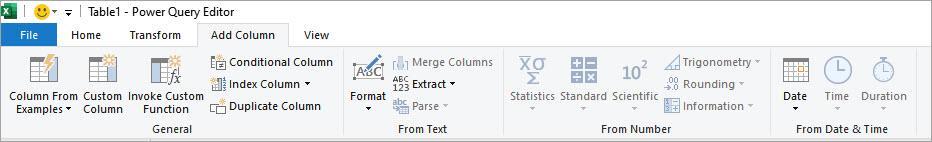
- Add Column tab – Use options on this tab to create new columns based on the existing data. For instance, you can create a new column using custom formulas, add a column based on conditions, and duplicate a column.
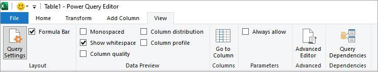
- View tab – Use options on this tab to customize the Power Query Editor’s layout and display features for working with queries. For instance, you can turn the Formula bar on and off to view and edit the M code for each step and open the Query Dependencies window to visualize how queries are linked.
- Query Pane – Lists all loaded queries in the workbook. The pane enables you to manage queries, such as renaming or duplicating them.
- Data Preview Pane – Displays a preview of your query’s data. Click the Data Type command button on the top left of a column header to expose options to change the column’s data type.
Click the Sort & Filter button in the top right of a column header to sort the column values in ascending or descending order and filter rows based on specific values.
Right-click a column header to display options to transform the column’s data.
- Formula Bar – Displays the M code (Power Query formula language) for the current transformation step. If you are familiar with the M language, you can write or edit expressions directly on the formula bar.
- Query Settings Pane – Has the Properties and Applied Steps sections. The Properties section displays the name of the selected query, which you can edit. It also allows you to add a description to the query. The Applied Steps section lists in a chronological order all the transformation steps you have applied to the query. When you select a query step, the data preview pane displays the data as it appeared up to and including that step.
- Status Bar – Displays information about the currently selected query, such as the number of columns and rows.
Refresh the Query
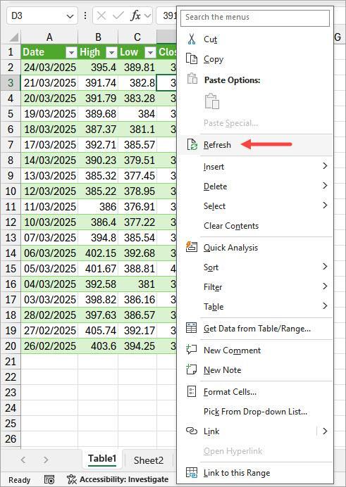
Power Query data is not directly linked to the source data. The query data is a snapshot of the data at the time of retrieval, meaning any changes in the source data will not automatically reflect in the Power Query data table. To update the data, you must manually refresh the query.
To refresh the query, right-click the results table and select the Refresh option on the shortcut menu.
How to Automate Refreshing Queries
You can automate refreshing queries to ensure you have the latest data.
Here’s how to do it:
1. Open the Data tab in Excel.
2. Click Queries & Connections on the Queries & Connections group.
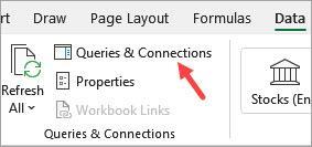
The above step opens the Queries & Connections pane to the right of the Excel window.
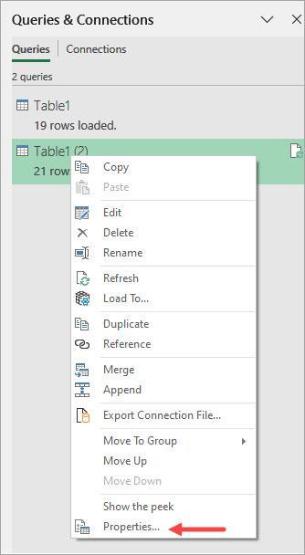
- Right-click the target Power Query data connection and select the Properties option on the shortcut menu.
The above step activates the Query Properties feature with the Usage tab open.
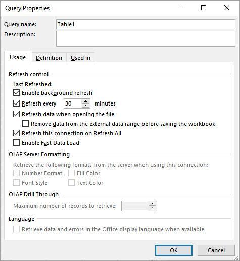
- Set your desired options for refreshing the target data connection. If, for instance, you select the ‘Refresh every X minutes’ option, Excel will automatically refresh the target data connection every specified number of minutes and refresh all tables connected to the connection. Even if you set a query to refresh automatically, you can refresh it manually whenever needed.
Managing Queries
As you add queries to the workbook, you will need a way to manage them. Excel offers the Queries & Connections pane for this purpose.
The Queries & Connections pane is particularly helpful when your workbook contains multiple queries. The pane functions like a table of contents, allowing you to locate and manage queries in your workbook.
You can open the Queries & Connections pane by opening the Data tab and clicking the Queries & Connections command button on the Queries & Connections group.

The above action opens the Queries & Connections pane to the right of the Excel window.
Right-click the query you want to work with and take any of the actions below.
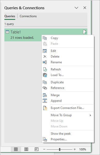
- Copy – Copy the query you have selected.
- Paste – Paste the query you have copied into the Queries & Connections in the current or another workbook.
- Edit – Open the Power Query Editor, where you can modify the query steps as explained in the section ‘Modify Query Steps on the Query Settings pane’ below.
- Delete – Delete the selected query. It cannot be undone.
- Rename – Rename the selected query.
- Refresh – Refresh the selected query’s data.
- Load To – Open the Import Data dialog box and redefine how you want to view and use the data in the workbook.
- Duplicate – Create an independent copy of the selected query. Changes you make to the duplicate query do not affect the original query.
- Reference – Create a new query that references the original query. Any changes you make to the original query will be reflected in the referenced query.
- Merge – Merge the selected query with another query in the Excel file by matching specified columns.
- Append – Append another query’s results in the workbook to the selected query.
- Export Connection File – Export the selected query with its referenced queries as an Office Data Connection (.odc) file for sharing with others.
- Move To Group – Move the selected query to a logical group you created for improved organization.
- Move Up – Move the selected query up one position on the query list, if possible. The option is unavailable if you have only one query.
- Move Down – Moves the selected query down one position on the query list, if possible. The option is unavailable if you have only one query.
- Show the Peek – Preview the results of the selected query.
- Properties – Open the Query Properties feature, where you can rename the selected query and add a description
Additional Actions
In the Power Query Editor, right-clicking a query in the Query pane on the left reveals three additional actions you can perform on it.
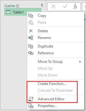
- Create Function – Convert the selected query into a function that can take parameters.
- Convert to Parameter – Convert the selected query into a parameter which can be used dynamically in other queries. The option is only available for queries with a single value input.
- Advanced Editor – Activate the Advanced Editor window to edit the query’s M code. The below screenshot of the Advanced Editor shows the M code of the example ‘Table1’ query in this tutorial.
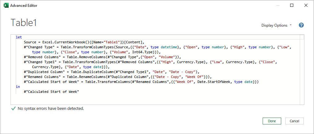
M language, also known as the Power Query Formula Language, is a functional and case-sensitive language used to transform data in Power Query.
M is declarative, focusing on defining the desired outcome rather than specifying how to achieve it. This makes M efficient for data extraction, filtering, transformation, and loading (ETL) tasks.
While Power Query automatically generates M code when you transform data on the Power Query Editor, the Advanced Editor allows you to modify the generated code.
Managing Query Steps
Once you have activated the Power Query Editor, select the target query on the Query pane on the left.
On the Applied Steps section of the Query Settings pane on the right, right-click any step and take any of the actions below.
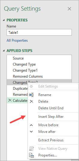
- Edit Settings – Modify the parameters or arguments defining the selected step. This option is available only for steps with configurable settings, such as those created through an interactive dialog box, like adding a custom column.
- Rename – Rename the selected step.
- Delete – Delete the selected step. Deleting a step can cause errors if subsequent steps depend on the removed step.
- Delete Until End – Delete the selected step and all subsequent steps.
- Insert Step After – Add a new step immediately after the selected step. Inserting a step between existing steps may affect subsequent steps and potentially break the query.
- Move Before – Move the selected step up one position, if possible.
- Move After – Move the selected step down one position, if possible.
- Extract Previous – Move all the steps before the one you have selected to a new query.
- View Native Query – Display the SQL query generated by the Power Query when connected to a database. This option is only available for database sources.
- Properties – Open the Step Properties feature to rename the selected step and add a description.
I have shown you all you need to get started with Power Query. I hope you found the tutorial helpful.
Other Power Query articles you may also like:
- Remove Null Values in Power Query
- Concatenate in Power Query (Columns, Text, Numbers)
- VLOOKUP in Power Query
- IF Then Else in Power Query
- Power Query Left Join
- Calculate Date Difference in Power Query (Days, Months, Years)
- Get Today’s Date in Power Query
- Find Maximum Value in a Column in Power Query
- Coalesce Operator in Power Query
- How to Undo in Power Query
- Power Query Functions List
Other Excel topics you may also be interested in: