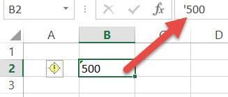
You might have come across Excel documents created by someone else that contains the apostrophe symbol in front of text, numbers, or dates.
You might have also noticed this happening when you copy tables or data from MS Word or import data from a webpage to the Excel worksheet.
Oftentimes, you don’t even realize they’re there because the apostrophes remain hidden and can only be seen when you see the cell contents in the formula bar.
If you’re curious to know what these apostrophes are for and how they can affect results of any subsequent actions applied to them, then read on.
In this Excel tutorial, I will not only be discussing what hidden apostrophes mean and why they are there, but I will also demonstrate three different and fool-proof ways to remove apostrophes in Excel.
So let’s get started!
Why Remove the Hidden Apostrophes in Excel – The Issue
Hidden apostrophes can often be a source of confusion and frustration because they cause cell contents to not behave the way you expect them to.
Sometimes they will not react to formatting, while other times you’ll find results of formulas applied to them not quite producing the expected result.
For example, consider the following table. You have here a set of numbers, the first four of which have leading apostrophes.
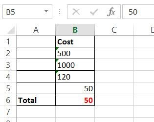
When you apply a calculation to this column, for example, the SUM function, notice it does not give the desired result.
You expect to get a sum of 1670, but the apostrophes have caused the SUM function to ignore the first 4 numbers and only consider the last number, 50.
Also read: How To Remove Formula From Excel
Why does the Apostrophe Appear?
Leading apostrophes forces excel to treat the cell’s contents as a text value. So, even if the cell contains a number or date, Excel will treat it as text.
But why would anyone want Excel to treat numbers or dates as text?
There can be many reasons for that.
If you specify something like Jan-01, Excel will automatically convert it to a date and format it according to your global date format (like 01/01/2020).
Go ahead and try it… It’s quite frustrating!
If you don’t want this to happen and you just want to display the text as ‘Jan-01’, then you need to somehow tell Excel that you want this to be considered as a text value, not as a date.
You can do so by simply adding a leading apostrophe.
Sometimes you might want leading zeros in your numerical values to remain. For example, you might have an ID number as:
000023452
If you don’t preface the number with an apostrophe, Excel will automatically format the number by removing all the leading zeros.
Also read: How to Add Zero In Front of Number in Excel (7 Easy Ways)
3 Ways to Remove Leading Apostrophes in Excel
If it’s just one or two cells, you can select the cell and remove the apostrophe to bring it back to normal.
However, if there’s a whole column of cells that you need to work with, then here are three ways to work around the problem:
Note: In case you’re thinking you can use Find and Replace to find the apostrophe symbol and replace it with a blank, it doesn’t work.
Using the Text-to-Columns Feature to Remove Apostrophe
This is the most commonly used method to remove leading apostrophes in Excel.
The Text-to-Columns feature is basically meant to help you split text contents in cells into multiple columns.
So, if you have a cell containing the full name of a person separated by a space, you can use the Text-to-Columns feature to separate the cell into two cells, one containing the first name and the other containing the last name.
During this process of splitting cells, the Text-to-Columns feature also converts numeric values to numbers, date values to dates, and all remaining values to text.
As such, this feature provides a really clever and quick way for you to convert all your apostrophe delimited cells back to their number or date formats.
Here’s how you can use this feature:
- Select the range of cells that you want to convert (remove apostrophes from).
- From the Data menu ribbon, select the ‘Text to Columns’ button.

- The ‘Convert Text to Columns’ wizard will appear. At this point, you don’t need to do anything more. Just press the Finish button directly.

That’s all!
You will see that all the leading apostrophes from the selected cells have been removed!
Also read: How to Add Text to End of Cells in Excel
Multiplying the Cells with 1
Here are another fool-proof method and quite a neat trick that you can use to remove leading apostrophes from cells containing numbers.
- Type the number 1 on any blank cell of your sheet.
- Press Ctrl+C to copy the value.
- Now select the range of cells that you want to convert (remove apostrophes from).
- Right-click and select ‘Paste Special’ from the popup menu that appears. This will open the Paste Special dialog box.
- Under ‘Operation’ you will find the ‘Multiply’ option. Select it and click OK. This will multiply every cell from your selected range with the number 1. The result is a set of the same numeric values, but with their apostrophes removed.
- You can delete the number 1 now because its job is done now.
Do remember though, this method only works with numeric values that contain leading apostrophes. This will not work with dates or text.
Also read: How to Remove Question Marks from Text in Excel?
Using VBA Code
The third way to remove apostrophes from any column in your sheet is to use VBA code. I would suggest you to go for this method only if you are a seasoned Excel user and don’t mind a little scripting to get the job done.
Here are the steps you need to follow:
- From the Developer Menu Ribbon, select Visual Basic.
- Once your VBA window opens, Click the Insert option in the menu and then click on Module. This will insert a new module in the project explorer pane

- Double click on the Module you just inserted in the Project Explorer. This will open the module code window.
- Type or copy-paste the following 6 VBA macro code lines into the module window:
Sub RemoveApostrophe()
With Worksheets("Sheet1").Columns(1)
.NumberFormat = "General"
.Value = .Value
End With
End Sub

Now depending on your requirement, you need to make two changes in line 2 of this code.
- You can replace “Sheet1” with the name of the sheet containing the cells you want to convert.
- Also, replace the number ‘1’ inside the Columns() functions with the number of the column you want to change. So Column A means 1, Column B means 2, and so on.
Once you have done the above steps, you’re all set to run the macro. And when you run this macro, it will instantly go to Column 1 and remove all the apostrophes from all the cells.
Below are the steps to Run the macro:
- Click anywhere in the code.
- Click on the green play/run button in the toolbar or press the F5 on your keyboard.
- Close the VBA window.
If you check your Excel Sheet now, you will find all the apostrophes removed and all the cells converted to the number format.
Note that if your column contains some date values with apostrophes and some without, this method might backfire, because it will convert the dates without apostrophes to a number, which, in the end, beats the purpose.
So these are the three methods you can use to remove hidden apostrophes from cells in Excel.
There are a number of other ways to do this too, but I found these 3 ways to be the most effective.
I hope you found this Excel tutorial useful.
Other Excel tutorials you may find useful:
- Excel Showing Formula Instead of Result (How to FIX!)
- How to Insert Square Root Symbol in Excel (5 Easy Ways)
- How to Clear Contents in Excel without Deleting Formulas
- How to Auto Format Formulas in Excel (3 Easy Ways)
- How to Convert Decimal to Fraction in Excel
- How to Remove Dollar Sign in Excel
- How to Remove Commas in Excel
- How to Remove Parentheses in Excel?
- How to Delete/Remove Checkbox in Excel?
Awesome tutorial…. big thumb UP.