When you’re working with data in Excel, sooner or later you will have to compare data. This could be comparing two columns or even data in different sheets/workbooks.
In this Excel tutorial, I will show you different methods to compare two columns in Excel and look for matches or differences.
There are multiple ways to do this in Excel and in this tutorial I will show you some of these (such as comparing using VLOOKUP formula or IF formula or Conditional formatting).
So let’s get started!
Compare Two Columns (Side by Side)
This is the most basic type of comparison where you need to compare a cell in one column with the cell in the same row in another column.
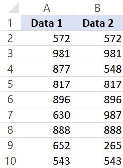
Suppose you have a dataset as shown below and you simply want to check whether the value in column A in a specific cell is the same (or different) when compared with the value in the adjacent cell.
Of course, you can do this when you have a small dataset when you have a large one, you can use a simple comparison formula to get this done. And remember, there is always a chance of human error when you do this manually.
So let me show you a couple of easy ways to do this.
Compare Side by Side Using the Equal to Sign Operator
Suppose you have the below dataset and you want to know what rows have the matching data and what rows have different data.
Below is a simple formula to compare two columns (side by side):
=A2=B2
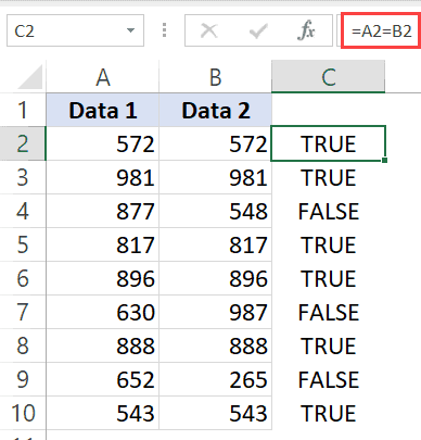
The above formula will give you a TRUE if both the values are the same and FALSE in case they are not.
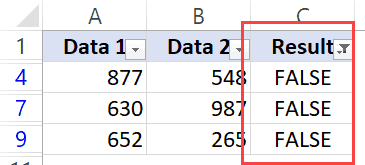
Now, if you need to know all the values that match, simply apply a filter and only show all the TRUE values. And if you want to know all the values that are different, filter all the values that are FALSE (as shown below):
When using this method to do column comparison in Excel, it’s always best to check that your data does not have any leading or trailing spaces. If these are present, despite having the same value, Excel will show them as different. Here is a great guide on how to remove leading and trailing spaces in Excel.
Compare Side by Side Using the IF Function
Another method that you can use to compare two columns can be by using the IF function.
This is similar to the method above where we used the equal to (=) operator, with one added advantage. When using the IF function, you can choose the value you want to get when there are matches or differences.
For example, if there is a match, you can get the text “Match” or can get a value such as 1.
Similarly, when there is a mismatch, you can program the formula to give you the text “Mismatch” or give you a 0 or blank cell.
Below is the IF formula that returns ‘Match’ when the two cells have the cell value and ‘Not a Match’ when the value is different.
=IF(A2=B2,"Match","Not a Match")
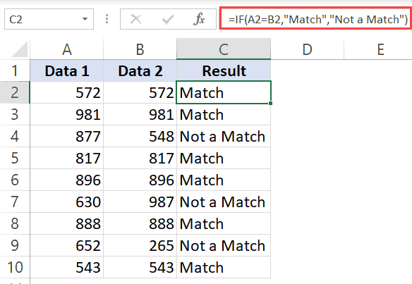
The above formula uses the same condition to check whether the two cells (in the same row) have matching data or not (A2=B2).
But since we are using the IF function, we can ask it to return a specific text in case the condition is True or False.
Once you have the formula results in a separate column, you can quickly filter the data and get rows that have the matching data or rows with mismatched data.
Also read: Does Not Equal Operator in Excel (Examples)
Highlight Rows with Matching Data (or Different Data)
Another great way to quickly check the rows that have matching data (or have different data), is to highlight these rows using conditional formatting.
You can do both – highlight rows that have the same value in a row as well as the case when the value is different.
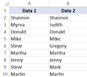
Suppose you have a dataset as shown below and you want to highlight all the rows where the name is the same.
Below are the steps to use conditional formatting to highlight rows with matching data:
- Select the entire dataset (except the headers)
- Click the Home tab
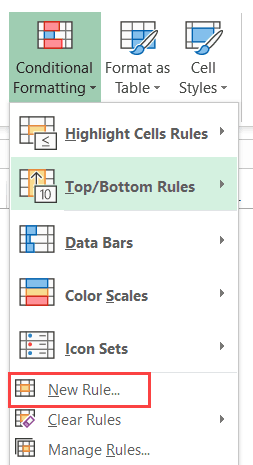
- In the Styles group, click on Conditional Formatting

- In the options that show up, click on ‘New Rule’
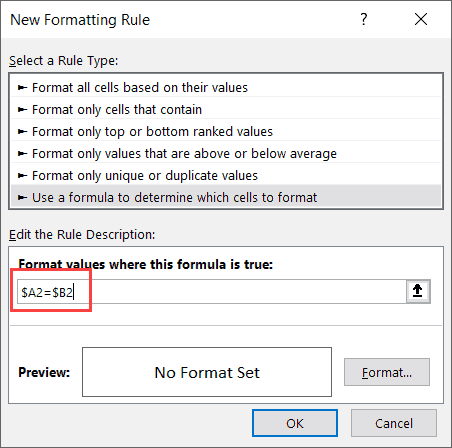
- In the ‘New Formatting Rule’ dialog box, click on the option -”Use a formula to determine which cells to format’
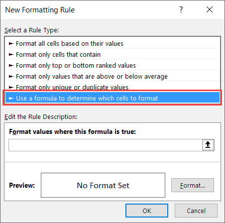
- In the ‘Format values where this formula is true’ field, enter the formula: =$A2=$B2
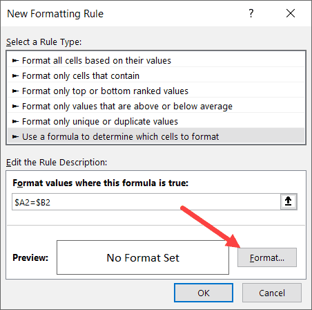
- Click on the Format button
- Click on the ‘Fill’ tab and select the color in which you want to highlight the rows with the same value in both columns
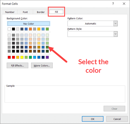
- Click OK
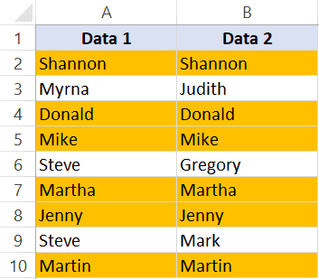
The above steps would instantly highlight the rows where the name is the same in both columns A and B (in the same row). And in the case where the name is different, those rows will not be highlighted.
In case you want to compare two columns and highlight rows where the names are different, use the below formula in the conditional formatting dialog box (in step 6).
=$A2<>$B2
How does this work?
When we use conditional formatting with a formula, it only highlights those cells where the formula is true.
When we use $A2=$B2, it will check each cell (in both columns) and see whether the value in a row in column A is equal to the one in column B or not.
In case it’s an exact match, it will highlight it in the specified color, and in case it doesn’t match, it will not.
The best part about conditional formatting is that it doesn’t require you to use a formula in a separate column. Also, when you apply the rule on a dataset, it remains dynamic. This means that if you change any name in the dataset, conditional formatting will accordingly adjust.
Compare Two Columns Using VLOOKUP (Find Matching/Different Data)
In the above examples, I showed you how to compare two columns (or lists) when we are just comparing side by side cells.
In reality, this is rarely going to be the case.
In most cases, you will have two columns with data and you would have to find out whether a data point in one column exists in the other column or not.
In such cases, you can’t use a simple equal-to sign or even an IF function.
You need something more powerful…
… something that’s right up VLOOKUP’s alley!
Let me show you two examples where we compare two columns in Excel using the VLOOKUP function to find matches and differences.
Compare Two Columns Using VLOOKUP and Find Matches
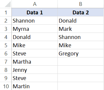
Suppose we have a dataset as shown below where we have some names in columns A and B.
If you have to find out what are the names that are in column B that are also in column A, you can use the below VLOOKUP formula:
=IFERROR(VLOOKUP(B2,$A$2:$A$10,1,0),"No Match")
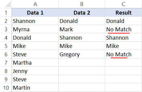
The above formula compares the two columns (A and B) and gives you the name in case the name is in column B as well A, and it returns “No Match” in case the name is in Column B and not in Column A.
By default, the VLOOKUP function will return a #N/A error in case it doesn’t find an exact match. So to avoid getting the error, I have wrapped the VLOOKUP function in the IFERROR function, so that it gives “No Match” when the name is not available in column A.
You can also do the other way round comparison – to check whether the name is in Column A as well as Column B. The below formula would do that:
=IFERROR(VLOOKUP(A2,$B$2:$B$6,1,0),"No Match")
Compare Two Columns Using VLOOKUP and Find Differences (Missing Data Points)
While in the above example, we checked whether the data in one column was there in another column or not.
You can also use the same concept to compare two columns using the VLOOKUP function and find missing data.
Suppose we have a dataset as shown below where we have some names in columns A and B.
If you have to find out what are the names that are in column B that not there in column A, you can use the below VLOOKUP formula:
=IF(ISERROR(VLOOKUP(B2,$A$2:$A$10,1,0)),"Not Available","Available")
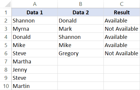
The above formula checks the name in column B against all the names in Column A. In case it finds an exact match, it would return that name, and in case it doesn’t find and exact match, it will return the #N/A error.
Since I am interested in finding the missing names that are there is column B and not in column A, I need to know the names that return the #N/A error.
This is why I have wrapped the VLOOKUP function in the IF and ISERROR functions. This whole formula gives the value – “Not Available” when the name is missing in Column A, and “Available” when it’s present.
To know all the names that are missing, you can filter the result column based on the “Not Available” value.
You can also use the below MATCH function to get the same result:
=IF(ISNUMBER(MATCH(B2,$A$2:$A$10,0)),"Available","Not Available")
Common Queries when Comparing Two Columns
Below are some common queries I usually get when people are trying to compare data in two columns in Excel.
Q1. How to compare multiple columns in Excel in the same row for matches? Count the total duplicates also.
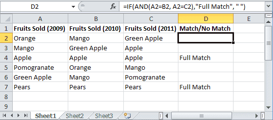
Ans. We have given the procedure to compare two columns in excel for the same row above. But if you want to compare multiple columns in excel for the same row then see the example
=IF(AND(A2=B2, A2=C2),"Full Match", "")
Here we have compared data of column A, column B, and column C. After this, I have applied the above formula in column D and get the result.
Now to count the duplicates, you need to use the Countif function.
=IF(COUNTIF($A2:$E2, $A2)=5, "Full Match", "")
Q2. Which operator do you use for matches and differences?
Ans. Below are the operators to use:
- To find matches, use the equal to sign (=)
- To find differences (mismatches), use the not-equal-to sign (<>)
Q3. How to compare two different tables and pull matching data?
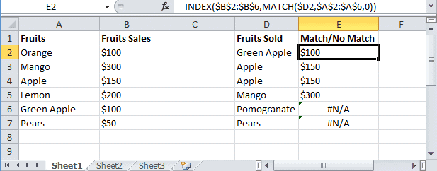
Ans. For this, you can use the VLOOKUP function or INDEX & MATCH function. To understand this thing in a better way, we will take an example.
Here, we will take two tables and now want to do pull matching data. In the first table, you have a dataset, and in the second table, take the list of fruits and then pull matching data in another column. For pull matching, use the formula
=INDEX($B$2:$B$6,MATCH($D2,$A$2:$A$6,0))
Q4. How to remove duplicates in Excel?
Ans. To remove duplicate data you need to first find the duplicate values.
To find the duplicate, you can use various methods like conditional formatting, Vlookup, If Statement, and many more. Excel also has an in-built tool where you can just select the data, and remove the duplicates from a column or even multiple columns
Q5. I can see that there is a matching value in both columns. However, the formulas you have shared above are not considering these as exact matches. Why?
Ans: Excel considers something an exact match when each and every character of one cell is equal to the other. There is a high chance that in your dataset there are leading or trailing spaces.
Although these spaces may still make the values seem equal to a naked eye, for Excel these are different. If you have such a dataset, it’s best to get rid of these spaces (you can use Excel functions such as TRIM for this).
Q7. How do we compare two columns that give the result as TRUE when all the first columns’ integer values are not less than the second column’s integer values? To solve this problem, I do not require conditional formatting, Vlookup function, If Statement, and any other formulas. I need the formula to solve this problem.
Ans. You can use the array formula for solving this problem.
The syntax is {=AND(H6:H12>I6:I12)}. This will give you “True” as a result whenever the value of Column H is greater than the value in Column I else “False” will be the result.
You may also like the following Excel tutorials:
- Compare Two Columns in Excel (for matches and differences)
- How to Remove Blank Columns in Excel? (Formula + VBA)
- How to Hide Columns Based On Cell Value in Excel
- How to Split One Column into Multiple Columns in Excel
- How to Select Alternate Columns in Excel (or every Nth Column)
- How to Paste in a Filtered Column Skipping the Hidden Cells
- Best Excel Books (that will make you an Excel Pro)
- How to Flip Data in Excel (Columns, Rows, Tables)?
- Find the Closest Match in Excel (Nearest Value)
- How to Compare Two Cells in Excel?
- VLOOKUP Not Working – 7 Possible Reasons + How to Fix!
- How to Group Duplicate Rows in Excel
What happened to Q6 and Answer.
Hi, does the VLOOKUP formula
=IF(ISERROR(VLOOKUP(B2,$A$2:$A$10,1,0)),”Not Available”,”Available”)
also work for date formats?