While Power Query lacks a direct equivalent to Excel’s VLOOKUP function, you can use its Merge feature to achieve the same result: locate a matching value in the leftmost column of a table and retrieve a corresponding value from a column you specify.
I will show you how to use the Power Query’s Merge feature to replicate the behavior of Excel’s VLOOKUP.
Suppose you have the Sales table below on the left and the Product table on the right on an Excel worksheet.
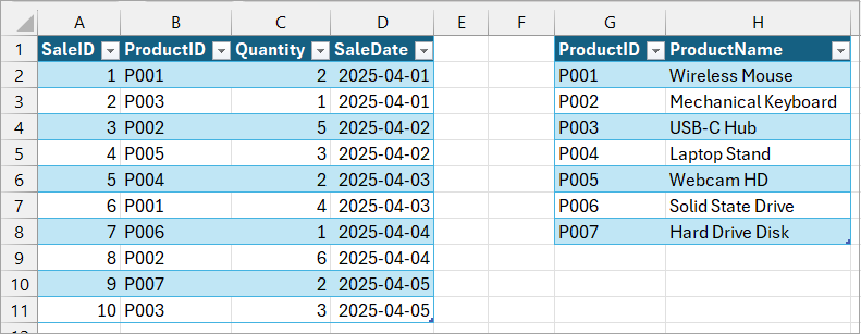
You want to use Power Query to add the ‘ProductName’ from the Products table to the Sales table by matching the ‘ProductID’ column, like how VLOOKUP works in Excel.
Here’s how to do it:
Step #1: Load the Data of Both Tables into Power Query Editor
Use the steps below to load the data of the Sales and Products tables into the Power Query Editor:
- Select any cell in the Sales table.
- Open the Data tab and click the From Table/Range command button.
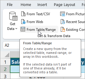
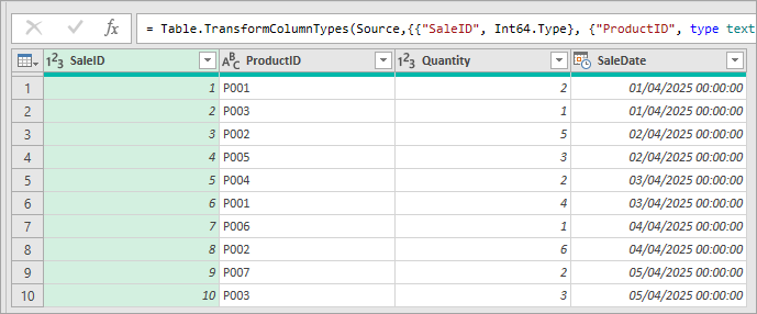
The above step loads the table data into the Power Query Editor.
- On the Home tab of the Power Query Editor, open the Close & Load drop-down on the Close group and select the Close and Load To option.
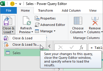
The above step opens the Import Data dialog box.
- On the Import Data dialog box, select the Only Create Connection option and click OK.
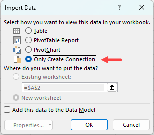
The above step loads the table data into the Power Query Editor for transformation without immediately loading it into an Excel worksheet or the data model.
- Load the Product table data onto the Power Query Editor using the steps above.
The queries you have created are listed on the Queries & Connections pane on the right of the Excel window.
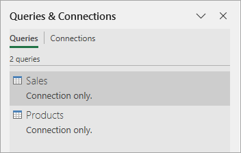
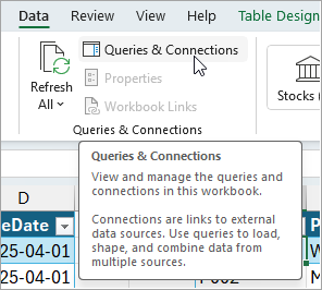
If you do not see the Queries & Connections pane, activate it by opening the Data tab and clicking the Queries & Connections command button on the Queries & Connections group.
Step #2: Merge the Queries
Use the steps below to merge the Sales and Products queries:
- On the Queries & Connections pane, right-click the Sales query and select the Merge option on the shortcut menu.
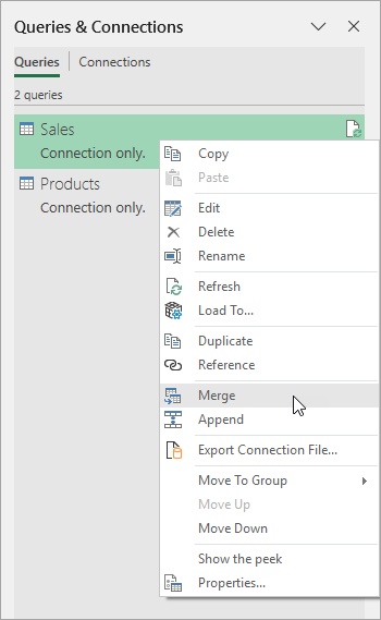
The above step opens the Merge dialog box with the Sales query already selected.
- On the Merge dialog box, open the second drop-down and select the Products query.
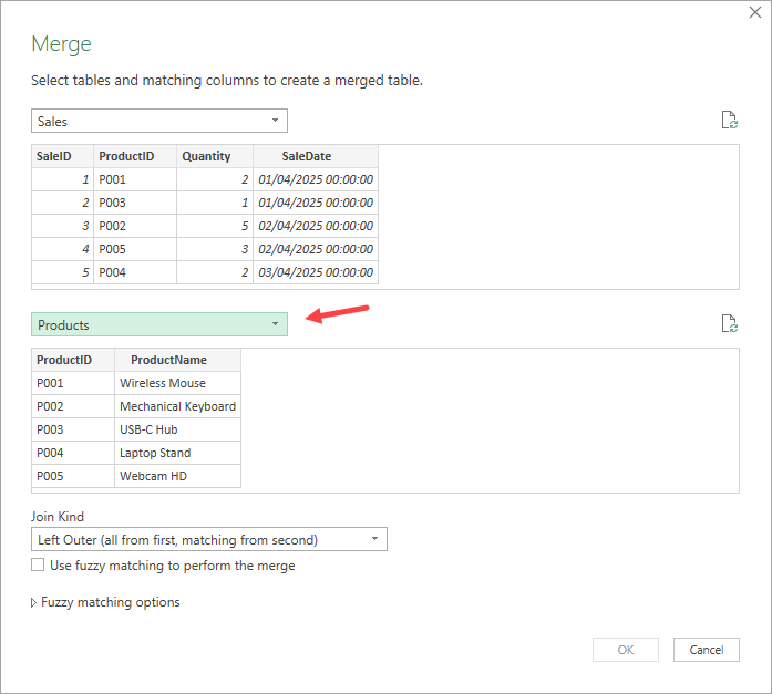
- Select the ProductID column in both queries, choose the ‘Left Outer’ join option, and click OK.
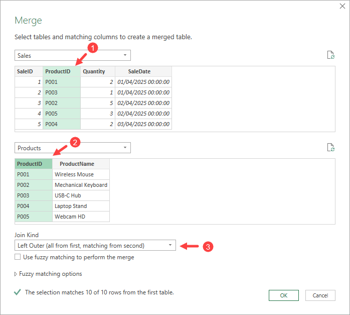
Note: A Left Outer join keeps all the rows from the left (primary) table, in this case the Sales table, and matches rows from the right (secondary) table, in this case the Products table, only when there’s a match. If no match is found, the result will include nulls for the columns from the right table.
The above steps merge the two queries into a Merge1 query and load it onto the Power Query Editor. The merged query has a Products column with a table icon on the left of the header.
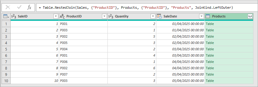
Notice the ‘expand column’ icon on the right of the Products column header.
Step #3: Expand the Target Column
Use the steps below to expand the ProductName column in the Merge1 query:
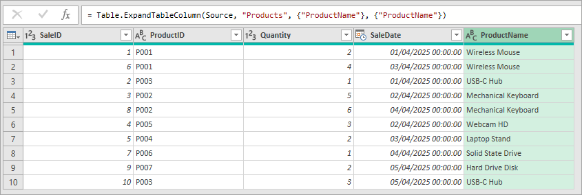
- Click the expand icon, uncheck the ‘Select All Columns’ option, select the ProductName column, uncheck the ‘Use original column name as prefix’ option, and click OK.
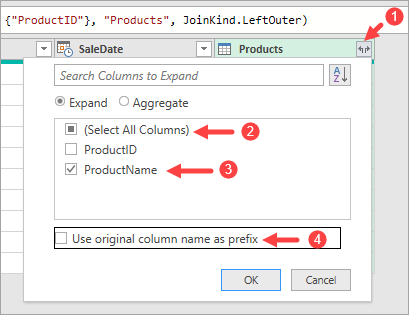
The above steps expand the ProductName column in the merged query.
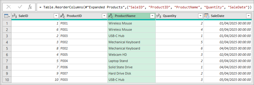
Move the ProductName column to the immediate right of the ProductID column by dragging its header.
Step #4: Load the Merged Query Data Back into Excel
Click the Close & Load button to load the merged query data back into Excel.
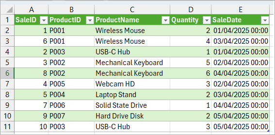
You have successfully done a VLOOKUP in Power Query using the Merge feature.
I have shown you how to do VLOOKUP in Power Query. I hope you found the tutorial helpful.
Other Power Query and Excel articles you may also like:
- Getting Started with Power Query
- Power Query Functions
- Remove Null Values in Power Query
- Concatenate in Power Query (Columns, Text, Numbers)
- Remove Duplicates in Power Query
- IF Then Else in Power Query
- VLOOKUP Not Working – Fix
- Using VLOOKUP Approximate Match in Excel
- Left Join in Excel Using Power Query