In Excel, the built-in Find and Replace feature works great when you need to find and replace a single value.
But if you’re dealing with multiple values at once, it’s not very practical.
The good news is, there are ways you can use to perform bulk find and replace—and that’s what I’ll show you in this tutorial.
Method #1: Using a Nested SUBSTITUTE Formula
The SUBSTITUTE function replaces specific text in a string with new text. When you nest it (use it inside another), each level replaces a different piece of text.
Example syntax:
=SUBSTITUTE(SUBSTITUTE(SUBSTITUTE(text, old_text1, new_text1), old_text2, new_text2), old_text3, new_text3)
In the example formula above:
- The first level SUBSTITUTE replaces old_text1 with new_text1.
- The second level SUBSTITUTE works on the above result and replaces old_text2 with new_text2.
- The third level SUBSTITUTE works on the above result and replaces old_text3 with new_text3.
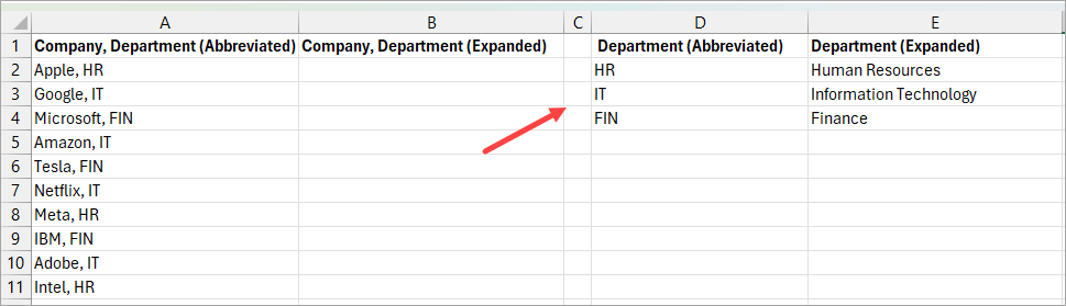
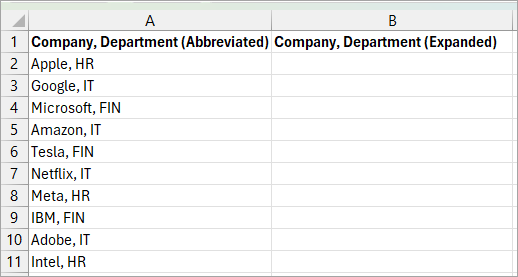
Suppose you want to replace the abbreviated department names in the cell range A2:A11 with full names and display the results in the cell range B2:B11.

Here’s how you can do it:
- Create a mapping table in another region of the worksheet, as in the example below.
- Enter the formula below in cell B2.
=SUBSTITUTE(SUBSTITUTE(SUBSTITUTE(A2:A11, D2, E2), D3, E3), D4, E4)
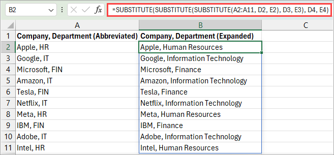
The formula replaces all abbreviated department names with full ones.
The formula only works in newer versions of Excel that support dynamic arrays. If you have an older version of Excel, modify the formula as follows:
=SUBSTITUTE(SUBSTITUTE(SUBSTITUTE(A2, $D$2, $E$2), $D$3, $E$3), $D$4, $E$4)
Using absolute references locks down the mapping table so that the references do not change when you copy the formula down the column.
Note: Press CTRL + SHIFT + ENTER to enter the formula because older versions of Excel do not support dynamic arrays.
Notes:
- The SUBSTITUTE function is case-sensitive, so ‘it’ won’t match ‘IT.’
- If you have many replacements to make, for example, ten or more, the formula becomes very long and unwieldy.
- Effective in replacing whole or parts of cell contents.
Method #2: Using the XLOOKUP Function
The XLOOKUP function looks for a specified value in a range or array and returns the corresponding value from another range or array.
You can apply the function in cases where you want to replace the entire contents of cells and not just parts of them.
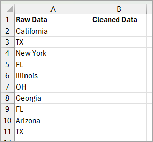
Suppose you have state names in column A and want to replace state abbreviations with full names and display the results in column B.
Here’s how you can accomplish it:
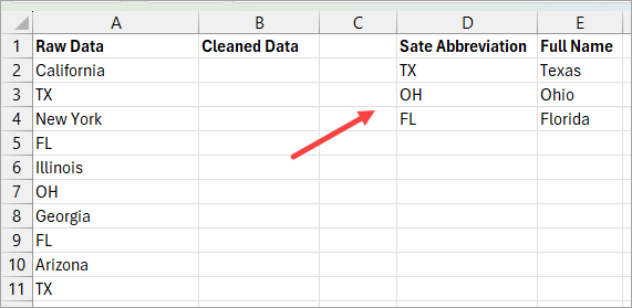
- Create a mapping table in another region of the worksheet, as in the example below.
- Enter the formula below in column B.
=XLOOKUP(A2, $D$2:$D$4, $E$2:$E$4, A2)
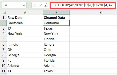
The formula replaces all state abbreviations with full names.
How the Formula Works
=XLOOKUP(A2, $D$2:$D$4, $E$2:$E$4, A2)
The formula looks up the value in cell A2 in the lookup array $D$2:$D$4. If it finds a match, it returns a corresponding value in the return array $E$2:$E$4. If it does not find a match, it returns the original value.
The XLOOKUP function is only available in newer versions of Excel.
If you have an older version of Excel, you can use a formula that combines VLOOKUP and IFNA or IFERROR functions, as shown in the example below.
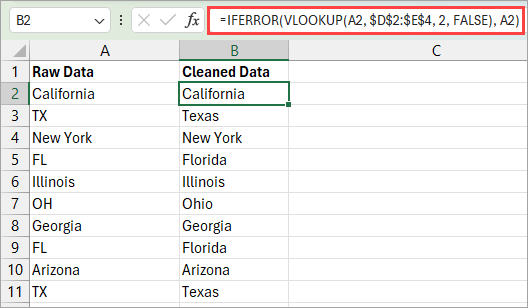
How the Formula Works
=IFERROR(VLOOKUP(A2, $D$2:$E$4, 2, FALSE), A2)
The formula looks up a value in cell A2 in the first column of the lookup range $D$2:$E$4. If it finds an exact match, it returns the corresponding value in the second column of the lookup range.
If it does not find an exact match, it returns the original value in cell A2 instead of an error.
Method #3: Use the REDUCE Function
Let’s say you want to replace the abbreviated department names in the cell range A2:A11 with full names and display the results in the cell range B2:B11.
You can use the REDUCE function to do the bulk find and replace operation. The REDUCE function lets you iterate over a range or an array and accumulate a single result by applying a custom LAMBDA calculation step by step.
Here’s how you can achieve that:
- Create a mapping table in another area of the worksheet, as in the example below.

- Enter the formula below in column B.
=REDUCE(A2:A11, SEQUENCE(ROWS(D2:D4)),LAMBDA(txt,i,SUBSTITUTE(txt, INDEX(D2:D4,i), INDEX(E2:E4,i))))
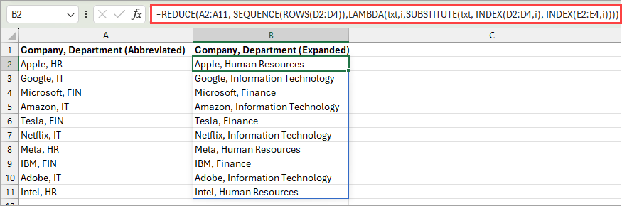
The formula iterates through each Find/Replace pair in D2:D4 and E2:E4, applying the SUBSTITUTE function to A2:A11 sequentially to replace all abbreviated department names with their full forms.
Method #4: Using VBA (by creating a UDF)
Let’s say you want to replace the abbreviated department names in the cell range A2:A11 with full names and display the results in the cell range B2:B11.

You can create a User-Defined Function in VBA and apply it to do the bulk find and replace operation.
Here’s how you can do it:
- Create a mapping table in another region of the worksheet, as in the example below.

- Copy the code below to a standard VBA module.
Function MASSFINDREPLACE(dataRange As Range, _
                              findRange As Range, _
                              replaceRange As Range) As Variant
    Dim arr() As Variant
    Dim result() As Variant
    Dim i As Long, j As Long
    Dim txt As String

    ' Load data into array for faster processing
    arr = dataRange.Value
    ReDim result(1 To UBound(arr, 1), 1 To 1)

    ' Loop through each row in data range
    For i = 1 To UBound(arr, 1)
        txt = arr(i, 1)

        ' Apply each find/replace pair to the current text
        For j = 1 To findRange.Count
            If j <= replaceRange.Count Then
                txt = Replace(txt, findRange.Cells(j, 1).Value, replaceRange.Cells(j, 1).Value)
            End If
        Next j

        result(i, 1) = txt
    Next i

    MASSFINDREPLACE = result
End Function- Enter the formula below in column B.
=MASSFINDREPLACE(A2:A11,D2:D4,E2:E4)
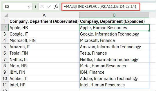
The formula replaces all the abbreviated department names with full names.
This VBA function that we have created performs bulk find and replace across a range of cells. It takes three inputs: a data range to modify, a list of text to find, and a list of replacement text. The function then loops through each cell in the data range and applies all find/replace pairs sequentially, then returns the modified results.
In this article, I’ve shown you four different methods you can use to do Find and Replace in bulk in Excel.
Of all the methods covered here, using the REDUCE function is going to be the most robust, as it can do the replacement across a range of cells as well as within the cell.
But if you just need to do one replacement per cell, then you can also use the XLOOKUP method or the SUBSTITUTE formula method.
And if this is something you need to do quite often, you can also rely on creating a simple VBA user-defined function.
Other Excel articles you may also like: