When you create a drop-down list in Excel, it only displays text options. But sometimes you may want it to show colors, too.
Although you can’t display colors in the drop-down list, you can still select an option and have the cell automatically change color (thanks to conditinal formatting).
I will show you how to create drop-downs that automatically change a cell’s color based on the selected value.
Creating Drop-down List with Color
Use the steps below to create drop-downs that change a cell’s color based on your selection.
Step #1: Create the Drop-down Lists
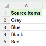
- Enter your drop-down source items in a range (A2:A5 in this case), on say, Sheet1.
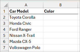
- On a different sheet, enter the dataset where you want to create the drop-downs.
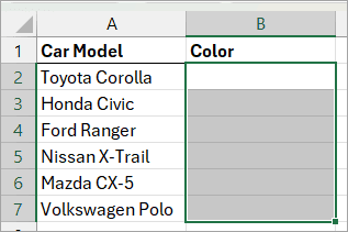
- Select the cell range where you want to create the drop-downs (B2:B7 in this case).
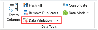
- Open the Data tab
- Click the Data Validation command button on the Data Tools group.
The above step opens the Data Validation dialog box.
- Do the following on the Data Validation dialog box:
- Open the Allow drop-down and select the List option.
- Enter the address of the cell range containing the source items on the Source box (=Sheet1!$A$2:$A$5 in this case).
- Click OK.

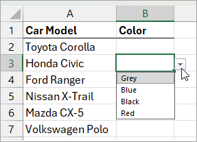
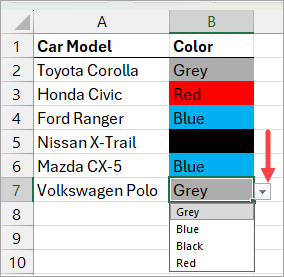
- Test the drop-downs by clicking the arrows next to the cells with the drop-down menus.
Step #2: Apply Conditional Formatting
Now that we have the drop-down list, let’s use conditional formatting to apply color to the target cell based on the selection.
Here’s how you do it:
- Select the cells with drop-down menus (B2:B7 in this case).
- Open the Home tab.
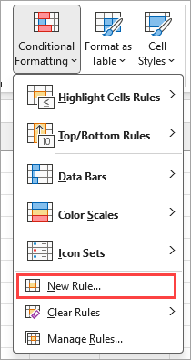
- Open the Conditional Formatting drop-down on the Styles group and select the New Rule option.
The above step opens the New Formatting Rule dialog box.
- Do the following on the New Formatting Rule dialog box:
- Click the ‘Format only cells that contain’ option on the ‘Select a Rule Type’ box.
- Open the first drop-down and select the ‘Specific Text’ option.
- Open the second drop-down and select the ‘containing’ option.
- On the box next to the drop-downs, enter the address of the first cell in the range containing the source items for the drop-downs you created in Step #1 (=Sheet1!$A$2 in this case).
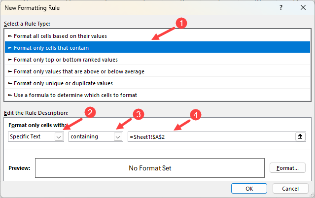
- Click the Format button.
The above step opens the Format Cells dialog box.
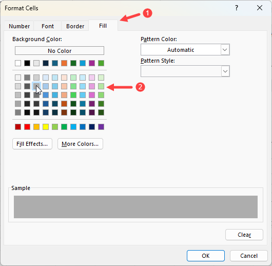
- Do the following on the Format Cells dialog box:
- Open the Fill tab.
- Choose a background color (Red in this case).
- Click OK.
After closing the Format Cells dialog box, Excel turns focus to the New Formatting dialog box.
- Review the settings you have applied on the New Formatting dialog box, then click OK.
- Repeat steps 1-9 above, choosing a different item in the source items list and the color that goes with it from the Format Cells dialog box.
Step #3: Test the Drop-downs
Test the drop-downs by clicking the arrows next to the cells with the menu items. After the drop-down selection, the target cell changes to the appropriate color.
Changing/Removing Colors in the Drop-down
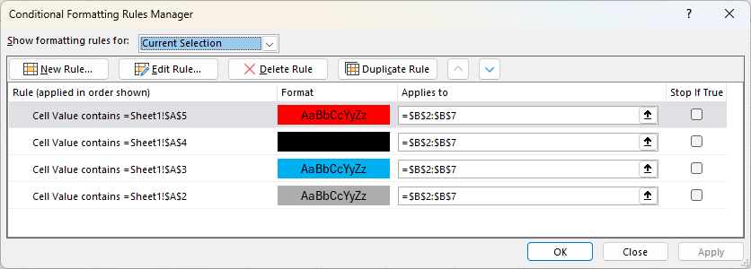
You can use the Formatting Rules Manager dialog box to review or edit the conditional formatting rules you have applied to your worksheet.
To open the Conditional Rules Manager:
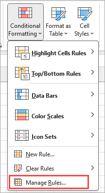
- Click the Home tab.
- Open the Conditional Formatting drop-down on the Styles group.
- Click the Manage Rules option on the drop-down list.
The above steps will open the Conditional Formatting Rules Manager dialog box.
I hope you found the tutorial helpful.
Other Excel articles you may also like: