When working with large data sets in Excel, it is often helpful to filter the data so that only the required rows are visible while the rest remain hidden.
While in most cases, users filter their dataset based on the cell’s values, Excel also allows you to filter your data by color. So you can choose what color cells should remain visible while the rest are filtered out and hidden.
Suppose we have a data set for the marks obtained by students in an exam, as shown below.
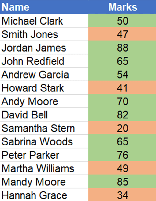
In this data set, students who have obtained passing marks have their cell color highlighted in green.
On the other hand, students who have failed the exam by not obtaining passing marks have their cell color highlighted in red. Obtaining marks greater than or equal to 50 is the passing criterion.
We may want to display the names of only those students who have passed the exam, or we may want to display the names of those who have failed the exam.
In either case, Excel provides a Filter by color feature to accomplish this easily.
So in this tutorial, I will show you different methods by which you can filter the data based on the color of a cell.
Method 1: Filter by Color Using the Filter Option
In this method, we will look at the Filter option to filter data based on a cell’s color. As an example, we will be using the student’s data set we saw earlier.

We will filter this data set to show only those cells that are highlighted in red (i.e., only show cells for students who failed the exam).
- Select the entire data set (including column headings). This will be from cells A1 to B15.

- Go to the Data tab.

- Under the ‘Sort and Filter’ section, click on the Filter button.

- Once you select the Filter button, a small arrow will appear next to each column heading, as shown below. This is where we will see the filter options.

- Click on the arrow next to the Marks column. (This is the column on which we want to filter the entire data set)

- The following menu will appear.

- From this menu, select the ‘Filter by Color’ option.

- The following sub-menu will appear.

You can see that both cell colors (red and green) appear in this Filter by Cell Color sub-menu. These colors are automatically shown based on the colors you have in the column.
- From this sub-menu, choose the red color option. (This is the color by which we want to filter our data).

- The result will look like the following.

You can see that the data has been filtered.
Rows that contain red cells are visible, whereas other rows are hidden.
So in this method, we have seen how to filter cells by color using the Filter option.
This method is helpful if you want to filter your data based on a single cell color. If you want to filter by multiple cell colors, you should look into Method 3 below.
Also read: How to Count Filtered Rows in Excel?
Method 2: Filter by Color Using the Right-Click Menu
In this method, we will look at the filter option available through the right-click menu to filter data based on a cell’s color.
As an example, we will be using the student data set we saw earlier. We will filter students whose marks are highlighted in red.

- Select cell B3. (This can also be any other cell in the column having the red color which we want to filter.)

- Right-Click in the selected cell. The context menu will appear as shown.

- From this menu, select the Filter option.

- A new window showing Filter options will appear as shown.

- From this window, select the Filter by Selected Cell’s Color option.

- The result will look like the one shown below.

As you can see, the data has been filtered. Rows, where the cell color is red, are visible, while the rest are hidden.
So in this method, we have seen how to filter cells by color using the Filter option available through the right-click menu.
This method is useful if you want to filter your data based on a single cell color. If you want to filter by multiple cell colors you should look into Method 3 below.
Also read: How to Create Custom Lists in Excel?
Method 3: Filter by Color Using the Sort Option
In this method, we will look at the Custom Sort option to filter data based on cell color.
Unlike the Filter option, sorting does not filter out data. Instead, data is sorted based on criteria.
Once the data is sorted, it becomes easier to examine, just like the filter option.
One advantage of using the Custom Sort Option is you can sort data based on multiple colors. This is not available with the Filter option (as you can filter data based on one color only).
As an example, take a look at the following data set.

This is the same data set as we saw in the previous example.
The only difference is that in this data set, students who have obtained more than 80 marks have their cell color highlighted in yellow.
We want to only see the students that have passed and have obtained more than 80 marks.
That is, we want to see students whose cell color is green or yellow.
We want to ignore students who have failed (in red color).
Let’s see the steps we need to take to achieve this result.
- Select the entire data set (including column headings). This will be from cells A1 to B15.

- Go to the Data tab.

- Under the ‘Sort and Filter’ section, click on the Sort icon.

- The Sort dialog box will appear as shown.

- Under the Sort by drop-down, select the Marks option. (This is the column on which we want to sort our data)

- Under the ‘Sort on‘ drop-down menu, select the Cell Color option.

- Under the Order drop-down menu, select the yellow color option. (This is the first color we want to appear on top)

- On the second drop-down option under the Order section, select the On Top option.

- Click on the Add Level button. (This will be our next sorting criteria.)

- A new level will be inserted as shown.

- Under the Then by drop-down menu, select the Marks option.

- Under the ‘Sort On‘ drop-down menu, select the Cell Color option.

- Under the Order, select the green color option. (This is the next color we want to appear on top after the previously selected yellow color)

- On the second drop-down option under the Order section, select the On Top option.

- Make sure that the option ‘My data has headers’ is checked. (If your data has column headings check this option, otherwise uncheck it)

- Click on OK.

- The result will look like the one below.

As you can see, the data has been sorted based on the two colors we have provided as our criteria. You can go ahead and hide rows 11 to 15 which are now easily selectable.
- Select rows 11 to 15 as shown.

- Right-Click anywhere inside the selected row to bring up the context menu.

- Select the Hide option.

- The end result will look as shown.

Now the data has been filtered as we wanted.
You can see that rows 11 to 15 are now hidden and that row 16 now appears after row 10.
Also read: VBA Codes to Filter Data In Excel
Method 4: Filter by Color Using VBA
If you are looking for a VBA script along with the AutoFilter function to filter data based on the color value of a cell, then this method may be useful.
As an example, we will be using the student data set we saw earlier in Method 1. We will filter students whose marks are highlighted in red.

- Open the VBA editor by pressing ‘Alt + F11’ on your keyboard. The following window will appear.

- From the menu bar at the top, click on Insert.

- Under the Insert menu, select the Module option.
- This will insert a new module where you can write your VBA script.

The VBA script to filter by color is shown below:
Sub Filter_By_Color()

StartRange = "A1"
RefCell = "B3"
RefColumn = 2
SheetName = "Sheet1"

Dim ws As Worksheet
Set ws = Worksheets(SheetName)

ws.Range(StartRange).AutoFilter field:=RefColumn, Criteria1:=Range(RefCell).DisplayFormat.Interior.Color, Operator:=xlFilterCellColor

End Sub
You’ll need to customize the above VBA code based on your own data. Here is the explanation of the above code.
StartRange: This is a user-defined variable that represents the start of the dataset that you want to filter. In this case, the sample dataset starts from cell “A1” which is why I have specified the value of StartRange equal to “A1”.
RefCell: This is a user-defined variable that specifies the cell whose color is to be taken as the filtering criteria. In this case, this is cell “B3”.
RefColumn: This is a user-defined variable that specifies the column number that needs to be filtered. In this case, it is 2, which is the Marks column.
SheetName: This is the name of the worksheet that contains the dataset. In this case, it is “Sheet1”.
- Copy and Paste the above VBA code into the module window.
- Bring the cursor on any line in the code and then press the ‘F5’. This will run the code instantly. (Alternatively, you can click on the green icon in the toolbar)

- You will see that the dataset has been filtered, as shown below.

So in this article, we have seen four methods of how to filter data based on cell color and an example showing how this can be useful.
Method 1 uses the Filter option to filter the data based on cell color. This method is, however, limited to filtering only one color.
Method 3 achieves the same effect as filtering using the Sort option and involves much more steps. But simultaneously, it allows you to filter data based on multiple cell color values.
For more advanced users who prefer using a VBA script, Method 4 is the way to go. VBA gives you a lot more control, and you can filter based on one or more colors.
Other Excel articles you may also like:
- How to Filter Multiple Columns in Excel? 3 Easy Ways!
- How to Clear Filter in Excel? Shortcut!
- Apply-Remove Filter In Excel (Shortcut)
- How to Change Cell Color Using VBA in Excel
- How to Paste in a Filtered Column Skipping the Hidden Cells
- How to Sort by Length in Excel? Easy Formula!
- How to Sort by Date in Excel (Single Column & Multiple Columns)
- How to Change Font Color Based on Cell Value in Excel?
- How to Change Theme Colors in Excel?
- Fill Color in Excel (Shortcut)
- Filter Strikethrough in Excel
- Count Colored Cells in Excel
- Create a Drop-down List with Color in Excel
- Excel Filter Not Working