SUMPRODUCT Function in Excel (5 Easy Examples)

If you want to multiply two or more lists of numbers together and add up the result in one go, the SUMPRODUCT function in Excel is exactly what you need.

It is one of those older functions that quietly does a lot, from weighted averages to conditional counts and sums without needing Ctrl+Shift+Enter.

Table of Contents

SUMPRODUCT Syntax

Here is the syntax of the SUMPRODUCT function:

=SUMPRODUCT(array1, [array2], [array3], ...)

array1 – The first array (or range) whose values you want to multiply and then add.
array2, array3, … – Optional. Additional arrays to multiply, position by position, before the totals are summed.

All arrays must have the same number of rows and columns. If they don’t match, SUMPRODUCT returns a #VALUE! error.

One thing worth knowing up front. SUMPRODUCT handles arrays natively, so you do not need to press Ctrl+Shift+Enter the way you used to with old array formulas. Just type the formula and hit Enter.

When to Use SUMPRODUCT

Use this function when you need to:

Multiply two columns (like quantity and price) and get the total in one step
Calculate a weighted average without breaking the formula into helper columns
Count or sum rows that meet multiple conditions, including OR logic
Reduce a spilled dynamic array to a single weighted total in one cell
Run array calculations in older Excel versions where SUMIFS or FILTER aren’t available

Let me show you a few practical examples of how to use SUMPRODUCT.

Example 1: Multiply Two Columns and Sum

Let’s start with the classic use case.

Below is a small bookstore inventory list with the title, copies in stock, and wholesale price per copy. I want the total value of the stock in a single cell.

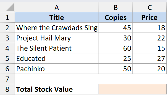
Excel table with book titles, copies, and prices, showing a blank cell for the Total Stock Value Sumproduct calculation

Here is the formula:

=SUMPRODUCT(B2:B6, C2:C6)

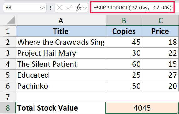
Excel formula bar showing =SUMPRODUCT(B2:B6, C2:C6) with a table of book titles, copies, and prices calculating 4045

In the above formula, SUMPRODUCT multiplies B2 by C2, B3 by C3, and so on down to B6 and C6. Then it adds up all those products and gives you a single total.

Without SUMPRODUCT you would need a helper column for copies × price and then a SUM at the bottom. This wraps both steps into one cell.

Example 2: Weighted Average with SUMPRODUCT

Here’s another practical scenario.

Say a recipe is being scored across three criteria, and each criterion carries a different weight (Flavor 50%, Texture 30%, Presentation 20%). You want the weighted average score for the dish.

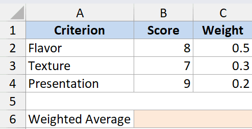
Sumproduct function example 2 showing a table with Criterion, Score, and Weight columns to calculate weighted average

Here is the formula:

=SUMPRODUCT(B2:B4, C2:C4) / SUM(C2:C4)

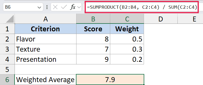
Excel formula bar showing SUMPRODUCT(B2:B4, C2:C4) / SUM(C2:C4) to calculate a weighted average from scores and weights

How this formula works:

SUMPRODUCT(B2:B4, C2:C4) multiplies each criterion’s score by its weight and adds the results.
SUM(C2:C4) adds up the weights (in this case 1 if you used decimals, or 100 if you used percentages as whole numbers).
Dividing one by the other gives you the weighted average.

If your weights already add up to 1 (for example 0.5, 0.3, 0.2), you can drop the divisor and just use =SUMPRODUCT(B2:B4, C2:C4). The math still works out.

Example 3: Count Rows Matching a Condition

This is the legacy power user trick that made SUMPRODUCT famous before COUNTIFS existed.

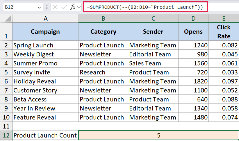
Below is a newsletter campaign log with the campaign name, category, sender, open count, and click rate. I want to count how many campaigns are tagged as the “Product Launch” category.

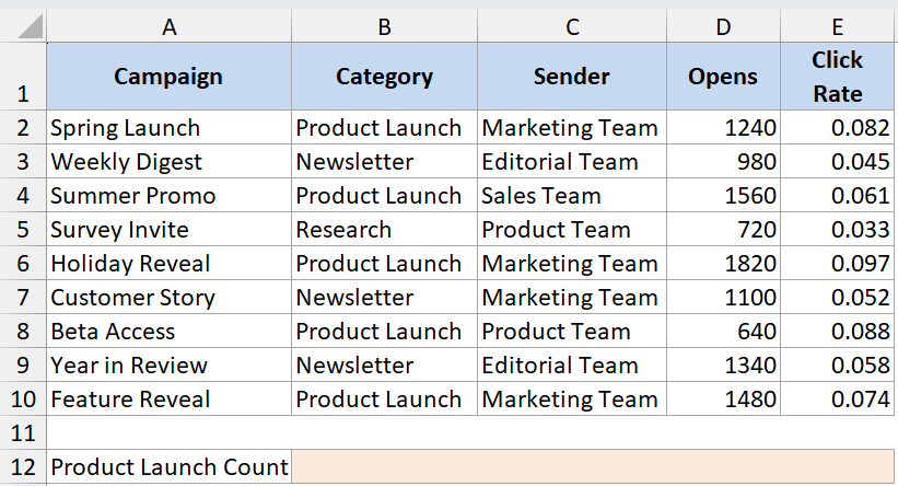
Sumproduct function example 3 showing an Excel table with campaign data and a Product Launch Count label in cell A12

Here is the formula:

=SUMPRODUCT(--(B2:B10="Product Launch"))

Excel formula bar showing SUMPRODUCT counting Product Launch entries in range B2:B10 with result 5 in cell B12

The B2:B10="Product Launch" part returns an array of TRUE/FALSE values. The double negative -- in front converts those to 1s and 0s. SUMPRODUCT then adds the 1s, giving you the count.

You could absolutely do this with COUNTIF today, and on Excel 365 you could also write =ROWS(FILTER(B2:B10, B2:B10="Product Launch")). The SUMPRODUCT version still has its uses though, especially when you want to combine the count with other calculations in the same formula.

Example 4: Conditional Sum Across Two Criteria

Now let’s step it up. I want to sum the open counts for campaigns where the category is “Product Launch” AND the sender is “Marketing Team”.

Excel table showing marketing campaign data with columns for Campaign, Category, Sender, Opens, and Click Rate

Here is the formula:

=SUMPRODUCT((B2:B10="Product Launch") * (C2:C10="Marketing Team") * D2:D10)

Excel formula bar showing SUMPRODUCT with two criteria to sum opens for Product Launch by Marketing Team

How this formula works:

(B2:B10="Product Launch") returns an array of TRUE/FALSE for each row’s category.
(C2:C10="Marketing Team") does the same check for the sender column.
Multiplying TRUE/FALSE arrays automatically coerces them to 1s and 0s, so you don’t even need the -- here.
The result of those two multiplications is multiplied by the open-count column. Rows that don’t match both conditions become 0 and drop out.
SUMPRODUCT adds whatever’s left.

This pattern is the SUMPRODUCT version of SUMIFS, and it works in every Excel version, including ancient ones that pre-date SUMIFS entirely.

In Excel 365 you can also write =SUM(FILTER(D2:D10, (B2:B10="Product Launch")*(C2:C10="Marketing Team"))), which often reads cleaner once you’re used to FILTER.

Example 5: OR Logic Across Two Columns

Here’s something SUMIFS struggles with. Say you want to count campaigns where the category is “Product Launch” OR the sender is “Marketing Team” (either one, not both required).

Sumproduct function example 5 showing an Excel table with campaign data including category, sender, opens, and click rate

Here is the formula:

=SUMPRODUCT(--((B2:B10="Product Launch") + (C2:C10="Marketing Team") > 0))

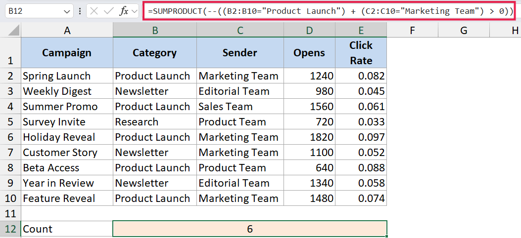
Excel formula bar showing SUMPRODUCT with OR logic for Product Launch and Marketing Team applied to campaign data table

In the above formula, adding the two TRUE/FALSE arrays gives you values of 0, 1, or 2 for each row. Wrapping it in > 0 flattens 1 and 2 back to TRUE, and the -- converts those to 1s for SUMPRODUCT to add.

OR logic across different columns is one of the spots where SUMPRODUCT still beats SUMIFS in everyday use.

The Excel 365 equivalent is =ROWS(FILTER(B2:B10, (B2:B10="Product Launch")+(C2:C10="Marketing Team"))), which uses the same + trick inside FILTER’s include argument.

When to Prefer SUMIFS or FILTER Instead

SUMPRODUCT is flexible, but it’s not always the right pick.

For straightforward conditional sums and counts, SUMIFS and COUNTIFS are easier to read and faster on big datasets. Reach for SUMPRODUCT only if you need OR logic or you’re stuck on an old Excel version.
For pulling matching rows out of a dataset, the FILTER function (Excel 365 and Excel 2021) is the modern answer. SUMPRODUCT can total things up, but it cannot return a list of matching records.
For reducing a spilled dynamic array to one number, you can wrap SUMPRODUCT around the spilled-range reference (=SUMPRODUCT(F2#, G2#)), but the simpler =SUM(F2# * G2#) usually does the same job in 365.
For very large datasets, SUMIFS tends to be more efficient because it processes the criteria more directly. SUMPRODUCT recalculates entire arrays.

If you need a side-by-side breakdown, the SUMPRODUCT vs SUMIFS comparison goes deeper on this.

Tips & Common Mistakes

Match your array sizes. All arrays inside SUMPRODUCT must have the same dimensions. A 5-row array multiplied by a 6-row array throws #VALUE!. Same applies if one is a row and the other is a column.
Watch for text in number ranges. If any cell in the array contains text (even a stray space), the multiplication may return #VALUE!. Clean the data first, or wrap the array in IFERROR if you’re stuck.
Use -- to coerce TRUE/FALSE. If your formula has only one logical test like (B2:B10="Product Launch"), you need -- to convert it. When you multiply two logical arrays with *, the multiplication does the coercion for you, so the -- becomes optional.
Don’t press Ctrl+Shift+Enter. SUMPRODUCT handles arrays natively. CSE was needed for old array formulas, not this one. In Excel 365 dynamic arrays have made CSE obsolete across the board, and SUMPRODUCT was already ahead of that change.
Avoid whole-column references like A:A inside SUMPRODUCT on large workbooks. It calculates across all 1,048,576 rows and slows things down. Use a tight range or a structured Table reference instead.
SUMPRODUCT pairs cleanly with spilled ranges. If you have a FILTER or SEQUENCE result spilling from F2, you can refer to it as F2# inside SUMPRODUCT (e.g. =SUMPRODUCT(F2#, G2#)) and the formula resizes automatically as the spill grows or shrinks.
Modern alternatives are often clearer. For “count where X” use COUNTIF/COUNTIFS. For “sum where X and Y” use SUMIFS. For OR logic or anything that needs to return rows, use FILTER. SUMPRODUCT remains useful for weighted averages and for legacy workbook compatibility.

SUMPRODUCT is older than most of the modern conditional functions, but it still handles a lot of work in a single cell, especially weighted averages and OR-logic counts. Once you get used to how arrays line up inside it, you’ll find yourself reaching for it more often than you’d expect, and you’ll know when to switch to FILTER or SUMIFS for a cleaner read.

List of All Excel Functions