SUMIFS Function in Excel

If you want to add up numbers based on more than one condition, the SUMIFS function in Excel is what you need.

In this article, I’ll show you how to use SUMIFS with multiple criteria, wildcards, comparison operators, and date ranges, plus how to combine it with dynamic arrays so a single formula returns one sum per category.

SUMIFS itself returns a single value, but it composes beautifully with the dynamic array tools in Excel 365. Feed it a spilled list of categories and you get a column of sums in one go, no copy-pasting required.

SUMIFS Syntax

Here is the syntax of the SUMIFS function:

=SUMIFS(sum_range, criteria_range1, criteria1, [criteria_range2, criteria2], ...)

• sum_range – The range of cells you want to add up.
• criteria_range1 – The first range to check against a condition.
• criteria1 – The condition to apply to criteria_range1.
• criteria_range2, criteria2 – Optional. Additional range/condition pairs. You can keep adding pairs up to 127 of them.

One quirk worth knowing right away. With SUMIFS, the sum_range is the first argument. With SUMIF, the sum_range is the last (and optional) argument. People who are used to SUMIF often trip on this when they switch to SUMIFS.

Also, SUMIFS uses AND logic. A row is included in the total only when every criteria is met. If even one condition fails, that row gets skipped.

When to Use SUMIFS

Use this function when you need to:

• Sum values that match two or more conditions at once
• Total amounts within a date range
• Sum numbers greater than, less than, or not equal to a value
• Add up values where the criteria contains a partial text match
• Produce a per-category breakdown by feeding SUMIFS a spilled list of unique categories

Let me show you a few practical examples of how this works.

Example 1: Sum Streaming Hours by User and Genre

Let’s start with a simple example.

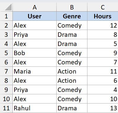
Below is a dataset with streaming history. Each row has a user, a content genre, and the number of hours watched. I want to find the total hours Alex spent watching Comedy.

Here is the formula:

=SUMIFS(C2:C11, A2:A11, "Alex", B2:B11, "Comedy")

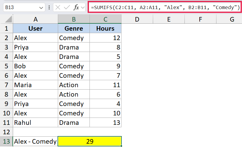
In the formula above, C2:C11 is the sum_range (the hours). The first criteria pair (A2:A11, “Alex”) checks the user column for “Alex”. The second pair (B2:B11, “Comedy”) checks the genre column. Only rows where both conditions are true get added.

Pro Tip: Text criteria always need to be inside double quotes. If you write Alex without quotes, Excel treats it as a name and the formula either errors out or returns 0.

Example 2: Sum Marathon Times Over a Threshold

Here’s another common scenario.

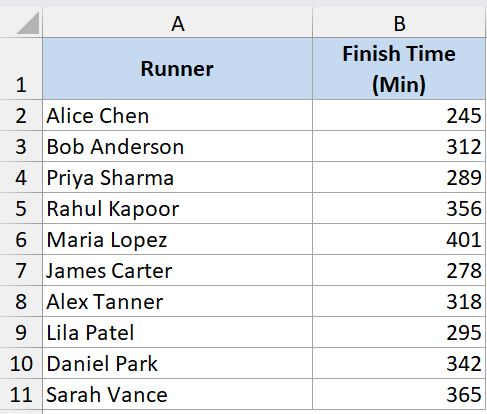
Say you have a list of runners and their marathon finish times in minutes, and you want to total the minutes for all runners who finished slower than 300 minutes.

Here is the formula:

=SUMIFS(B2:B11, B2:B11, ">300")

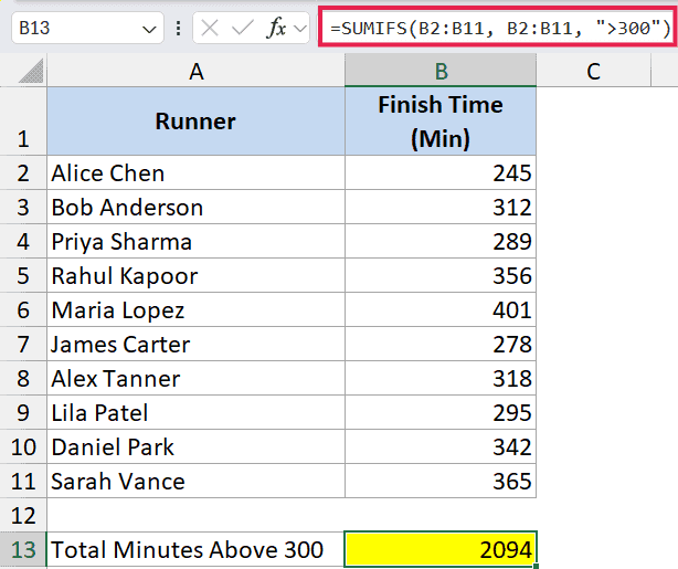
Notice that the sum_range and criteria_range are the same (B2:B11). That is fine. SUMIFS lets you use the same range for both when the condition you’re checking is on the values you’re summing.

The criteria ">300" has to be wrapped in quotes. The greater-than sign followed by the number is treated as one piece of text. The same rule applies to "<100", ">=50", or "<>0" (not equal to zero).

If you want to compare against a number stored in a cell instead of a hardcoded value, use this format:

=SUMIFS(B2:B11, B2:B11, ">"&D2)

The & joins the operator and the cell reference into a single criteria string.

Example 3: Sum Donations With a Wildcard

Now let’s look at something a bit more interesting.

You have a list of donor organizations and their donation amounts, and you want to total contributions from every group that has the word “Trust” anywhere in its name (Children’s Trust, Heritage Trust Fund, Trust for Conservation, etc.).

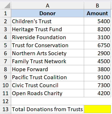
Here is the formula:

=SUMIFS(B2:B11, A2:A11, "*Trust*")

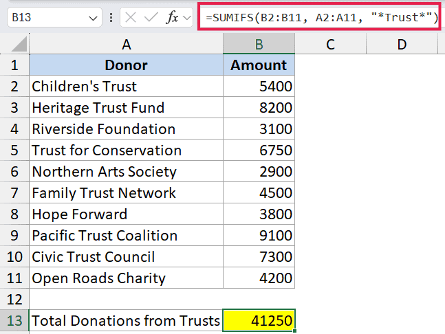
The asterisk (*) is a wildcard that matches any number of characters. So "*Trust*" matches anything that has “Trust” somewhere in it.

A few wildcard variations:

• "Trust*" matches text starting with Trust (Trust for Conservation).
• "*Trust" matches text ending with Trust (Children’s Trust).
• "?ond" matches four-character strings ending in “ond” (Bond, Pond, Fond).

One thing to note. Wildcards only work on text values. If you try to use them on numbers, they won’t match anything.

Example 4: Sum Within a Date Range

This is one I use quite often.

Below is a dataset with emergency room visit dates and treatment costs. I want to total all costs for visits between January 1, 2025 and March 31, 2025.

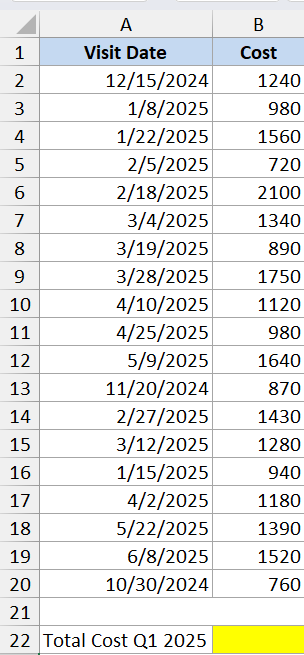
Here is the formula:

=SUMIFS(B2:B20, A2:A20, ">="&DATE(2025,1,1), A2:A20, "<="&DATE(2025,3,31))

Two criteria pairs are doing the work here. The first one checks that the date is on or after January 1, 2025. The second checks that the date is on or before March 31, 2025. Both have to be true for a row to be counted.

I’m using the DATE function to build the dates because it avoids regional formatting issues. If you write ">=1/1/2025" directly, Excel may read it as January 1 in some locales and as something else in others. DATE is bulletproof.

You can also reference cells that hold the start and end dates:

=SUMIFS(B2:B20, A2:A20, ">="&D2, A2:A20, "<="&D3)

Where D2 has the start date and D3 has the end date.

Example 5: Per-Category Spilled Sums With Dynamic Arrays

Let’s step it up with the most useful pattern in modern Excel.

Say you have a long list of expenses with a category column and an amount column, and you want a clean breakdown of total spend per category. Pre-365, you’d type SUMIFS once and copy it down. In Excel 365, you can do the whole thing in two formulas that spill automatically.

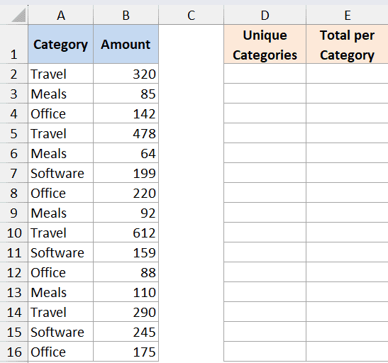
Start by spilling the unique categories with UNIQUE:

=UNIQUE(A2:A16)

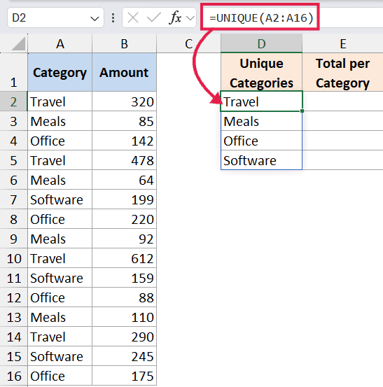
If that lands in cell D2, the spilled range is D2#. Now use SUMIFS with D2# as the criteria, and SUMIFS spills one sum per category alongside it:

=SUMIFS(B2:B100, A2:A100, D2#)

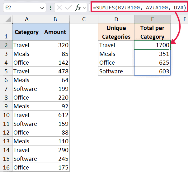
Here, the criteria argument isn’t a single value any more. It’s a spilled array of categories from D2#. SUMIFS evaluates each one in turn and returns a parallel array of sums, which spills down next to the categories.

Add a new row to the source data with a new category, and both spills extend automatically. No copy-pasting, no formula maintenance. This is the pattern to reach for whenever you’d previously have built a pivot table just for a quick subtotal view.

SUMIFS vs SUMIF

These two are easy to mix up, so here’s the short version.

• SUMIF sums based on a single condition. Syntax: =SUMIF(range, criteria, [sum_range]). The sum_range is the last argument and is optional.
• SUMIFS sums based on one or more conditions. Syntax: =SUMIFS(sum_range, criteria_range1, criteria1, ...). The sum_range is the first argument and is required.

SUMIFS can do everything SUMIF does. So if you only ever remember one of them, remember SUMIFS. The argument order is different, but it handles single-criteria cases just fine.

If you’re choosing between SUMIFS and SUMPRODUCT for more flexible logic (like OR conditions), I have a separate write-up on that here: SUMPRODUCT vs SUMIFS Function in Excel.

Tips & Common Mistakes

• Feed it a spilled array for per-category sums. As shown in Example 5, passing D2# (or any spilled range) as the criteria turns SUMIFS into a one-formula breakdown. Pair with UNIQUE for the categories and SORT if you want them ordered.
• Range sizes must match. Every criteria_range and the sum_range have to be the same shape and size. If sum_range is B2:B11 and criteria_range is A2:A20, you’ll get a #VALUE! error. Always double-check that all ranges cover the same number of rows.
• Text criteria need quotes. Writing Alex without quotes makes Excel think it’s a defined name. Use "Alex". Same goes for operators: ">500" not >500.
• Use & to join operators with cell references. If your threshold lives in a cell, write ">"&D2 not ">D2". Without the &, Excel reads the whole thing as literal text.
• Wildcards don’t work on numbers. They only match text. If your numbers are stored as text (look for the green triangle in the corner), wildcards may suddenly start working, which is usually a sign your numbers are in the wrong format.
• SUMIFS uses AND logic only. Every condition has to be true for a row to count. If you need OR logic (e.g., sum where category is either “Travel” OR “Meals”), add two SUMIFS together or switch to SUMPRODUCT.
• <> excludes a value. To total everything except a specific name, use "<>Alex" as the criteria. Combine with other pairs the usual way.
• Watch for hidden spaces. Criteria like "Alex" won’t match "Alex " (with a trailing space). If your formula returns 0 when you expect a number, run TRIM on the data column.
• Use DATE() for date criteria. It avoids regional date format issues and makes the formula portable across machines.
• Watch out for @ in older workbooks. When a workbook saved by Excel 2019 or earlier opens in 365, Excel sometimes auto-inserts an @ symbol (e.g. =@SUMIFS(...)) that collapses any spilled criteria back to a single value. Remove the @ and the spill returns.

Once you get the hang of the argument order and the quoting rules, SUMIFS handles pretty much every conditional sum you’ll run into.

The single-cell version covers the basics, and the spilled-criteria pattern in Example 5 turns it into the modern replacement for a quick pivot-table summary. Pair it with UNIQUE and SORT and you’ve got a live, formula-driven breakdown of any dataset.

List of All Excel Functions