If you want to find where a specific piece of text sits inside a longer string, the SEARCH function is what you’re looking for. It returns the position of the substring as a number, and it’s case-insensitive, so “PRO”, “Pro”, and “pro” all match the same way.
In Excel 365, you can also feed SEARCH a range and the results will spill into the cells below.
In this article, I’ll show you how the SEARCH function works, along with its syntax and a few practical examples that you can use right away.
SEARCH Function Syntax
Here is the syntax of the SEARCH function:
=SEARCH(find_text, within_text, [start_num])
- find_text – The text you want to find. Wildcards (
?and*) are allowed. - within_text – The text you want to search inside.
- start_num – Optional. The character position in
within_textwhere the search should begin. Defaults to 1 if you skip it.
If SEARCH cannot find the text, it returns a #VALUE! error.
When to Use SEARCH
Use this function when you need to:
- Find where a keyword or character appears inside a longer text string
- Check whether a cell contains a specific word, regardless of letter casing
- Pull out part of a string based on the position of a marker character
- Use wildcards to match a flexible pattern instead of an exact phrase
- Skip past the first occurrence of a character and find a later one
Let me show you a few practical examples so the function actually clicks.
Example 1: Find Position of a Character
Let’s start with something simple.
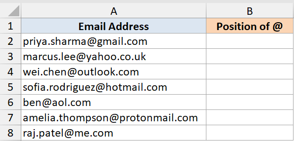
Below is the dataset. Column A has a list of email addresses. I want to know the position of the @ character in each one.
The @ sits at a different spot in every email because usernames have different lengths, so this is a clean way to see SEARCH locating the same character at different positions.
Here is the formula:
=SEARCH("@", A2:A8)
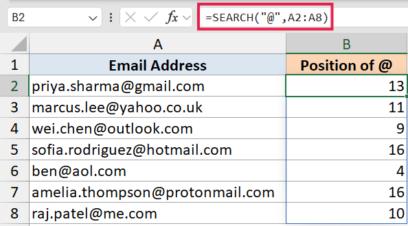
Since I’m in Excel 365, the formula spills down the column on its own, so a single entry in cell B2 fills the whole result range.
Knowing the position of the @ symbol is also the first step if you ever want to pull out the username (everything before the @) or the domain (everything after). That’s a common follow-up task and the next example shows the same “find a delimiter, then extract” pattern in action.
Pro Tip: If you only need a yes or no answer (rather than the position), wrap SEARCH inside ISNUMBER. That converts the position number into TRUE and the #VALUE! error into FALSE, which is much friendlier to work with. Example 3 shows that pattern.
Example 2: Extract First Name from Full Name
Here’s another scenario you’ll run into all the time.
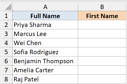
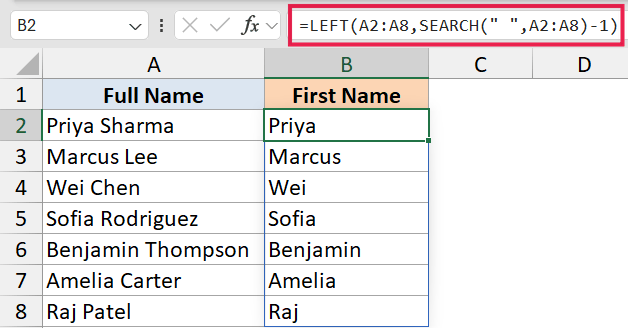
Below is the dataset. Column A has a list of full names. I want to pull out just the first name from each row.
The trick is that first names are different lengths, so I can’t just grab a fixed number of characters. I need to know where the space sits in each name, then take everything to the left of it.
Here is the formula:
=LEFT(A2:A8, SEARCH(" ", A2:A8) - 1)
How this formula works:
SEARCH(" ", A2:A8)finds the position of the first space in each name.- Subtracting 1 from that position gives us the number of characters before the space (the first name).
LEFT(...)then pulls out exactly that many characters from the left.
The formula spills down the column in Excel 365, so one entry in B2 fills all the results.
If you’re on Excel 365, you can also do this more directly with TEXTBEFORE: =TEXTBEFORE(A2:A8, " ") returns everything before the first space in one step. The SEARCH + LEFT approach still works (and works in older Excel versions where TEXTBEFORE doesn’t exist), so it’s worth knowing both.
Caveat: This formula assumes every row has at least one space. If a row has only a single word (no space), SEARCH(" ", ...) returns a #VALUE! error. You can wrap the whole thing in IFERROR to handle that case, or use IF to check for a space first.
Example 3: Flag Rows Containing a Keyword
This one comes up a lot when you’re working with free-form text like reviews or feedback.
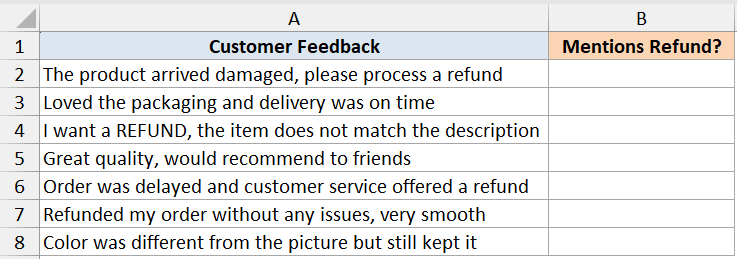
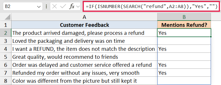
Below is the dataset. Column A has a list of customer feedback messages, and I want to flag every row that mentions the word “refund” so I can deal with those rows first.
The keyword can sit anywhere in the sentence and the casing won’t be consistent either, so I need a check that doesn’t care about position or case.
Here is the formula:
=IF(ISNUMBER(SEARCH("refund", A2:A8)), "Yes", "")
How this formula works:
SEARCH("refund", A2:A8)returns a number when “refund” is found in the cell, or a#VALUE!error when it isn’t.ISNUMBER(...)converts that into TRUE (number) or FALSE (error).IF(...)then returns “Yes” for TRUE and a blank for FALSE.
Because SEARCH ignores case, “Refund”, “REFUND”, and “refunded” all get picked up by the same formula. You don’t have to write separate conditions for each spelling.
This is the cleanest way to ask “does this cell contain a specific word?” in Excel, and you can apply it to any keyword you care about. It’s also the building block for a partial-match COUNTIF when you want to count rows that mention a keyword.
Example 4: Extract Middle Name Using start_num
Here’s a scenario where the optional third argument of SEARCH earns its keep.
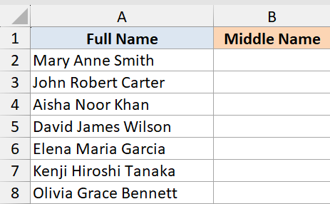
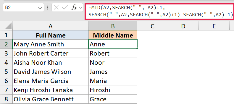
Below is the dataset. Column A has a list of full names that include a middle name, and I want to pull out just the middle name from each row.
The trick is that I need to find both the first space and the second space in each name, then take everything between them. The start_num argument is what lets me skip past the first space and find the second one.
Here is the formula:
=MID(A2, SEARCH(" ", A2) + 1, SEARCH(" ", A2, SEARCH(" ", A2) + 1) - SEARCH(" ", A2) - 1)
How this formula works:
SEARCH(" ", A2)finds the position of the first space.SEARCH(" ", A2, SEARCH(" ", A2) + 1)usesstart_numto start searching one position after the first space, so it returns the position of the second space.- Subtracting one from the other tells me how many characters sit between the two spaces, minus 1 to leave the second space out.
MID(...)then extracts that chunk, starting one position after the first space.
Without start_num, there’s no clean way to find the second occurrence of a character — SEARCH would always return the first one. So this is where the third argument really pays off.
If you’re on Excel 365, you can also use TEXTSPLIT to break the name into pieces and grab the middle one: =INDEX(TEXTSPLIT(A2, " "), 2). That’s cleaner when you just want the middle name. The SEARCH + start_num approach earns its keep when you need fine control over which occurrence to pick, or when you’re working in older Excel where TEXTSPLIT isn’t available.
Caveat: This formula assumes every row has at least two spaces (i.e. a first, middle, and last name). If a row has just a first and last name, the inner SEARCH returns a #VALUE! error. Wrap the formula in IFERROR if you want to handle those rows gracefully.
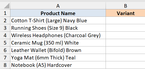
Example 5: Extract Text Inside Parentheses
Let’s wrap up with a more advanced use case.
Below is the dataset. Column A has a list of product names, and each name has the variant (size, color, or pack size) inside parentheses. I want to pull out just the text between the parentheses.
The trouble is that the parentheses sit at different spots in each row, and the text inside is different lengths. So I need to find both the opening and the closing parenthesis, then take whatever lives between them.
Here is the formula:
=MID(A2, SEARCH("(", A2) + 1, SEARCH(")", A2) - SEARCH("(", A2) - 1)
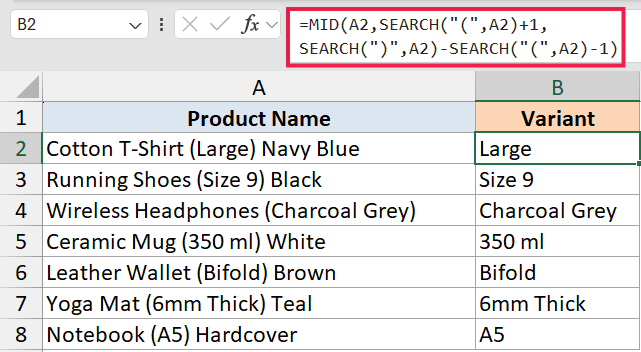
How this formula works:
SEARCH("(", A2)finds the position of the opening parenthesis.SEARCH(")", A2)finds the position of the closing parenthesis.- Subtracting one from the other tells me how many characters sit between them, minus 1 to leave the closing parenthesis out.
MID(...)then extracts that chunk of text, starting one position after the opening parenthesis.
You can drag this formula down the column, or in Excel 365 swap A2 for A2:A8 to get the spilled version.
If you’re on Excel 365, you can also do this with TEXTBEFORE and TEXTAFTER nested together: =TEXTBEFORE(TEXTAFTER(A2, "("), ")"). That reads more naturally than the MID + SEARCH version, and you don’t have to count offsets. The MID + SEARCH approach still works in older Excel, so it’s worth knowing both.
Caveat: This assumes every row has a pair of parentheses. If a row is missing one or both, SEARCH returns a #VALUE! error. Wrap the formula in IFERROR if you want to return a blank in those rows instead.
Tips & Common Mistakes
- SEARCH is not case-sensitive. If you need a case-sensitive match, use FIND instead. FIND has the same syntax but treats “A” and “a” as different characters.
- Wildcards are supported in SEARCH but not in FIND. A
?matches any single character and a*matches any sequence. SoSEARCH("a?c", A2)finds “abc”, “axc”, “a9c”, etc. To search for a literal?or*, put a tilde~right before it. - The
#VALUE!error means the substring wasn’t found. Don’t panic when you see it. Wrap SEARCH in IFERROR or ISNUMBER depending on what you want to do with the missing rows. - In Excel 365, you don’t need to drag the formula down. Pass SEARCH a range and the results spill automatically. The older “Ctrl + Shift + Enter” approach for array behavior is no longer needed in modern Excel.
- If you’re on Excel 365, the newer text functions are worth knowing too. TEXTBEFORE, TEXTAFTER, and TEXTSPLIT cover several of the extraction patterns above more directly. SEARCH is still essential when you need the actual position number, when you need fine control with
start_num, or when you’re working in an older Excel version where the new functions don’t exist.
In this article, I covered how the SEARCH function works in Excel, along with its syntax and five practical examples to show how it behaves in real situations.
Once you get the hang of SEARCH, you’ll find yourself reaching for it inside formulas with MID, LEFT, RIGHT, IF, and ISNUMBER all the time, especially when you need to extract part of a text string in your data.
Related Excel Functions / Articles: