If you’re an Excel user, you’ve probably heard of wildcards.
Wildcards are special characters that allow you to perform “fuzzy” matching on text in your formulas.
You can use them to find and replace text, match patterns, and more. In this section, we’ll cover the available wildcards, for example, wildcard usage and functions that support wildcards.
Available Wildcards in Excel
Excel has three wildcards you can use in your formulas:
- Asterisk (*)
- Question mark (?)
- Tilde (~)
The asterisk represents zero, one, or more characters, the question mark represents any single character, and the tilde is used as an escape character for literal characters such as ~* for a literal asterisk, ~? for a literal question mark, or ~~ for a literal tilde.
Note that wildcards only work with text, not numbers.
Example Wildcard Usage
Here are some examples of how you can use wildcards in your formulas:
| Usage | Behavior | Will Match |
|---|---|---|
| ? | Any one character | “A”, “B”, “c”, “z”, etc. |
| ?? | Any two characters | “AA”, “AZ”, “zz”, etc. |
| ??? | Any three characters | “Jet”, “AAA”, “ccc”, etc. |
| * | Any characters | “apple”, “APPLE”, “A100”, etc. |
| *th | Ends in “th” | “bath”, “fourth”, etc. |
| c* | Starts with “c” | “Cat”, “CAB”, “cindy”, “candy”, etc. |
| ?* | At least one character | “a”, “b”, “ab”, “ABCD”, etc. |
| ???-?? | 5 characters with hyphen | “ABC-99″,”100-ZT”, etc. |
| *~? | Ends with a question mark | “Hello?”, “Anybody home?”, etc. |
| *xyz* | Contains “xyz” | “code is XYZ”, “100-XYZ”, “XyZ90”, etc. |
Remember that wildcards only work with text. For numeric data, you can use logical operators.
Functions that Support Wildcards
Not all functions allow wildcards, but here is a list of the most common functions that do:
- AVERAGEIF, AVERAGEIFS
- COUNTIF, COUNTIFS
- MATCH
- MAXIFS, MINIFS
- SEARCH
- SUMIF, SUMIFS
- VLOOKUP, HLOOKUP
- XLOOKUP
- XMATCH
By using wildcards, you can make your Excel formulas more powerful and flexible. Whether you’re finding and replacing text or matching patterns, wildcards can help you get the job done.
Let me show you some examples on how to use Wildcards in Excel
Wildcard Characters Examples in Excel
Let’s now have a look at some examples of using Wild Characters in Excel and how it can help you be more efficient in your day-to-day work.
Use Wildcard Characters to Filter Data
Below, I have a dataset where I have the product codes in column A and the sales values in column B.

Now, assume that I want to filter product codes that start with the letter “A”.
To do that, I can follow the below simple steps.
- Click on the filter icon in the “Product code” header. So, click the filter icon on cell A1.
- Then, type “A*” in the filtering field.
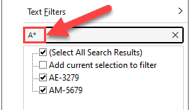
- Click “OK”.

Now, I have filtered product codes that start with the letter “A”.

If you have not used the asterisk sign, then Excel filters all product codes that contain the letter “A” anywhere of the product code. So, you’ll also get “SA-1036” in the filtered list.
In this case, the “Asterisk” sign (*) after the letter A helped you to filter product codes that start with the letter “A”. The Asterisk sign represents any number of characters.
But, if you want to specify the number of characters, you can use the question marks instead of the asterisk. Each question mark represents any single character.
Below, I have a dataset where I have the product codes in column A and the sales quantity in column B.

Now, I want to filter product code with four characters.
To do that, I can easily use wildcards for filtering.
- Click on the filter icon in the “Product code” header. So, click the filter icon on cell A1.
- Type “????” (four question marks) in the filtering field. If you want to filter codes with five characters, you have to type five question marks because each question mark represents one character.
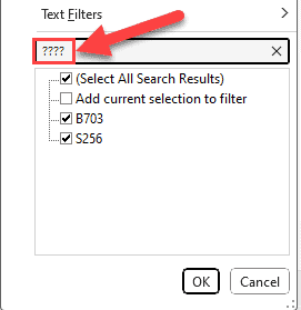
- Click “OK”.

Now, you have filtered product codes with four characters.

Sometimes, we want to filter items that contain an asterisk (*) or question mark (?).
For example, if you want to filter items with an asterisk sign, you can’t just enter the asterisk sign to filter the data. Let’s look at the below example.
Below, I have a dataset where I have the product codes in column A and the sales quantity in column B. An asterisk is used at the end of the product codes to identify high-value products.

Now, I want to filter high-value products.
To do that, I have to follow the steps below.
- Click on the filter icon in the “Product code” header. So, click the filter icon on cell A1.
- Type “~*” (A tilde followed by an asterisk) in the filtering field. When I use the tilde mark (~), Excel reads the next character as it is and not as a wildcard character. So, if I want to filter items with a question mark, I have to use “~?”.

- Click “OK”.

Now, you have filtered product codes with an asterisk sign.

Wildcard Characters to Find and Replace Partial Matches
You can also use Excel wildcard characters to Find and Replace.
Below, I have a dataset where I have the names in column A and the country in column B.

You can notice that I have written “the United States” with different abbreviations. Now, I want you to keep one abbreviation format for all records.
I can follow the below steps for that.
- Select the Country column. So, I select column B data.

- Press “Ctrl + H” to open the “Find and Replace” dialog box.
- Enter “U*” on the “Find What” box.

- Enter the preferred abbreviation for the United States in the “Replace with” box. So, I enter “USA” in the “Replace

- Click “Replace All”.

Now, you can see all the abbreviations of the United States in the same format.

Using Wildcard Characters Inside Excel Functions
You can use the wildcard characters when you want to do partial matches, such as XLOOKUP, VLOOKUP, SUMIF, and many other functions.
Below, I have a dataset where I have the product codes in column A and the sales values in column B.
Now, I want to find the total sales product codes that start with the letter “A”.
For that, I can use the below formula.
=SUMIF(A2:A6,"A*",B2:B6)

In the above formula, I have used the wildcard – asterisk (*) to create a condition with a partial match.
The XLOOKUP function has the ability to do a lookup based on wildcard characters.
Below, I have a dataset where I have the product codes in column A and the sales quantity in column B.
Now, I want to get the product code that starts with the letter “A” and has 3 characters only.
To do that, I can use the below XLOOKUP formula.
=XLOOKUP("A??",A2:A6,A2:B6,,2)
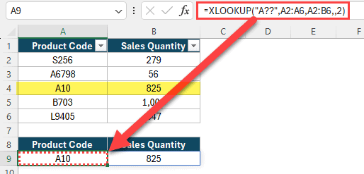
In the above formula, I have used “A??” for the lookup_value argument. It helps me to look up codes that have only three characters and also start with the letter A.
Whenever you are using wildcard characters in your XLOOKUP formula, you have to set the match mode argument to number 2.
Using Wildcard Characters with Conditional Formatting
Sometimes, we have to use wildcards to apply conditional formatting.
Below, I have a dataset where I have the product codes in column A and the sales quantity in column B. An asterisk is used at the end of the product codes to identify high-value products.
Now, I want to apply conditional formatting to highlight high-value product rows.
For that, I can follow the below steps.
- Select the entire data table without headers.

- Go to the “Home” tab.

- Go to the “Styles” group and expand the “Conditional Formatting” options. Then, click “New Rule…”.

You’ll get the “New Formatting Rule” dialog box.
- Select “Use a formula to determine which cells to format”.

- Enter the below formula as the rule.
=ISNUMBER(SEARCH("~*",$A2))

- Click the Format button and select the way you want to format cells that meet the given criteria.

- Click the “OK” button.
Now, I have highlighted all the high-value product rows in my table.

In this article, I covered everything you need to know about wild card characters, including some practical examples of using them in Excel spreadsheets.
Other Excel articles you may also like: