If you want to repeat a piece of text inside a cell a set number of times, the REPT function is what you need.
It is a small text function, but people use it for a surprising number of things. Padding IDs with leading zeros, building tiny in-cell bar charts, and even tricks like pulling the last text value out of a column.
In Excel 365, you can also feed REPT a range and the results spill into the cells below.
In this article, I’ll walk you through how REPT works with a few practical examples.
REPT Function Syntax in Excel
Here is the syntax of the REPT function:
=REPT(text, number_times)
- text – The text string you want to repeat. This can be a literal string in quotes, a cell reference, or a formula that returns text.
- number_times – A positive number that tells Excel how many times to repeat the text. If it is zero, REPT returns an empty string. If it is not a whole number, Excel truncates the decimal part.
A quick caveat. The result of REPT cannot be longer than 32,767 characters. If you push past that limit, you get a #VALUE! error.
When to Use REPT
Use this function when you need to:
- Build a quick in-cell bar chart without inserting a real chart object
- Pad numbers or IDs with leading zeros or other characters so they line up
- Create star ratings, tally marks, or dot charts inside a cell
- Add a visual separator line between sections of a report
- Generate a long string of the same character for spacing or formatting
Let me show you a few practical examples of how to use REPT.
Example 1: In-Cell Bar Chart for Survey Scores
Let’s start with the most popular use of REPT, building a tiny bar chart inside a cell.
Below is the dataset. I have a list of product features in column A and an average customer rating out of 100 for each feature in column B.
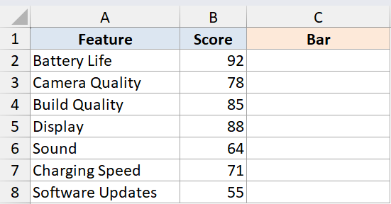
I want a visual bar next to each score so I can scan the strongest and weakest features at a glance, without inserting a real chart.
Here is the formula:
=REPT("|",B2:B8/5)
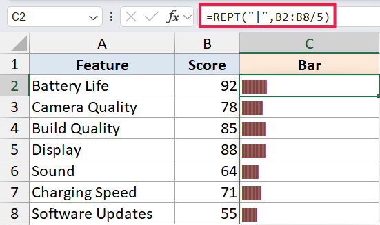
Here, REPT repeats the pipe character once for every 5 points in the score.
Since I am feeding it the entire range B2:B8 in one shot, the formula spills the bars down column C automatically. Dividing by 5 keeps the bars at a reasonable width inside the cell.
To make this look more like a real chart, change the font of the result column to a narrow font like Playbill or Stencil, and set the font color to the color you want for the bars. You can also use conditional formatting on the score column to color the bars based on thresholds.
Pro Tip: Pick the divisor based on your range of values. For scores out of 100, dividing by 3 or 5 gives a comfortable bar width. For values in the thousands, divide by 50 or 100 to keep the bar inside the cell.
Example 2: Pad Customer IDs with Leading Zeros
Here’s another practical scenario, lining up short numbers so they all have the same width.
Below is the dataset. I have raw customer IDs in column A that came out of a system without padding, so some are 1 digit and others are 4 digits.
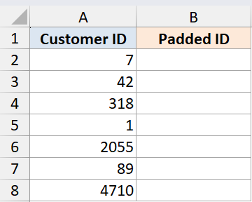
I want every ID to be 5 digits wide, with zeros added to the front of the shorter ones.
Here is the formula:
=REPT("0",5-LEN(A2:A8))&A2:A8
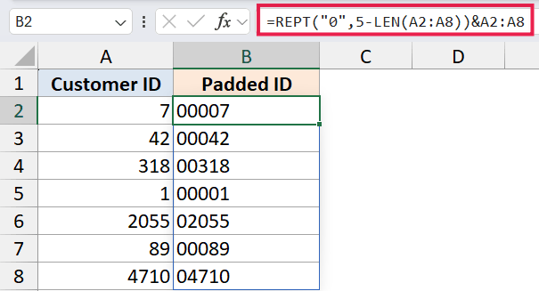
How this formula works:
- LEN(A2:A8) returns the length of each ID in the range.
- 5 minus that length tells REPT how many zeros it needs to add.
- REPT then builds a string of zeros that long, and the ampersand glues those zeros to the front of the original ID.
The whole thing spills down column B in one go.
In Excel 365, you can also do this with TEXT in many cases: =TEXT(A2:A8, "00000"). That is cleaner when your IDs are pure numbers. The REPT version is more flexible though, since it handles mixed text and numbers without complaining about format codes. For other approaches, see our full guide on add leading zeros in Excel.
A quick caveat. If an ID is already longer than 5 characters, the formula returns an error because REPT cannot accept a negative count. Wrap it in MAX if your data has that risk: =REPT("0", MAX(0, 5 - LEN(A2:A8))) & A2:A8.
Example 3: Add a Separator Line Between Sections
Now let’s look at something simpler. Sometimes you want a clean horizontal line between sections of a report without messing with borders.
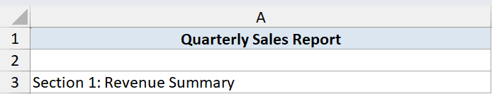
I have a report header in cell A1 and a section title in A3. I want a divider line in A2.
Here is the formula in A2:
=REPT("-",80)
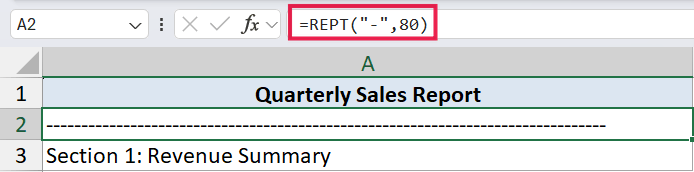
This just spits out 80 dashes in a row. It is a single-cell formula, so there is no spill to worry about here. You can swap the dash for an equals sign, an underscore, or any character that fits your style. This is also a quick way to add text or symbols across a range of cells when you want consistent formatting.
Pro Tip: If you change the row above or below frequently and want the line to match the column width, multiply by a column-width estimate instead of hardcoding 80. For most fonts, the cell width in pixels divided by 7 is close enough.
Example 4: Build a Star Rating Display
Let’s step it up with a more visual example. Star ratings are everywhere on review sites, and you can build the same look inside a cell.
Below is the dataset. I have product names in column A and a rating from 1 to 5 in column B.
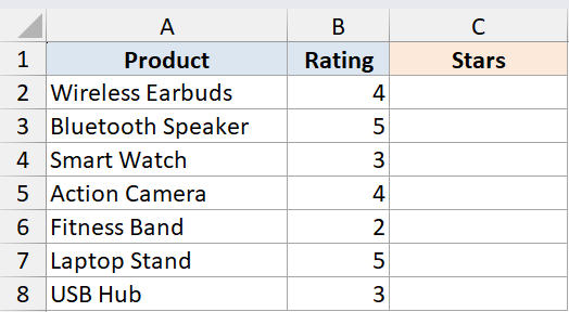
I want to show full stars for the rating and empty stars for the rest, so each row has exactly 5 stars total.
Here is the formula:
=REPT("★", B2:B8) & REPT("☆", 5 - B2:B8)
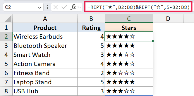
How this formula works:
- The first REPT repeats the filled star symbol the same number of times as the rating.
- The second REPT repeats the hollow star for the remaining slots out of 5.
- The ampersand joins them into one string per row.
Since I am passing the whole B2:B8 range, the formula spills the star strings down the column in one shot.
Pro Tip: You can swap the symbols for any Unicode characters. Try ● and ○ for dots, ▰ and ▱ for filled and empty bars, or ✓ and ✗ for pass/fail. Just paste the character inside the quotes.
A quick caveat. This works best when ratings are whole numbers. For half-star ratings, you would need a third REPT for a half-star symbol like ½ or a separate INT and MOD calculation.
Example 5: Find the Last Text Entry in a Column
This last one is a clever trick that uses REPT in a way you would not expect. It finds the last text value in a column, even when the column has gaps.
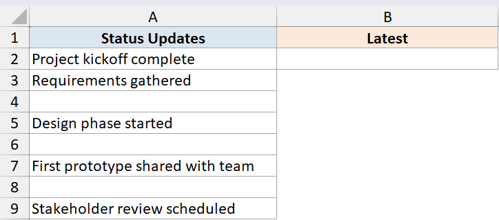
Below is the dataset. I have a list of status updates in column A, with some blank cells mixed in. The list grows over time, and I want to always pull the most recent entry.
Here is the formula:
=VLOOKUP(REPT("z", 255), A:A, 1)
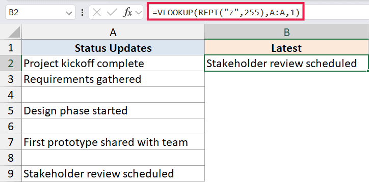
How this formula works:
- REPT builds a string of 255 lowercase z’s, which is alphabetically larger than any realistic text value.
- VLOOKUP looks for that huge string in column A with the default approximate match behavior.
- Since no value is actually larger, VLOOKUP returns the last text value it scanned before giving up, which is the last text entry in the column.
This is handy for dashboards where you want a “latest status” cell that always points to the most recent text in a log.
A quick caveat. This only works for text values. If you need the last number in a column, use =LOOKUP(2, 1/(A:A<>""), A:A) instead.
Tips & Common Mistakes
- The result cannot exceed 32,767 characters. If your formula returns #VALUE!, that is almost always the cause. Reduce the repeat count.
- A negative
number_timesargument also throws #VALUE!. Wrap the count in MAX(0, …) when there is any chance it could go negative. - Decimal repeat counts are truncated, not rounded.
=REPT("X", 3.9)returns “XXX”, not “XXXX”. - REPT is case sensitive on the text input.
=REPT("a", 3)and=REPT("A", 3)give different results. - For in-cell charts, pick a font that has equal-width characters, like Stencil, Playbill, or any monospace font. Variable-width fonts make the bars look uneven.
- In Excel 365, you can feed REPT a range argument and it spills automatically. In older versions like 2019 and 2016, you would need to enter it as one of the array formulas with Ctrl+Shift+Enter or copy the formula down manually.
That covers what REPT does and the most common ways to use it. The function itself is small, but it gets you a long way when you need quick visuals or text padding. Try it the next time you want a tiny bar chart inside a dashboard or need to line up IDs in a column.
Related Excel Functions / Articles:
- Microsoft Excel Terminology (Glossary)
- ASCII in EXCEL
- How to Concatenate with Line Breaks in Excel?
- Control E in Excel – What Does it Do?
- Bulk Find and Replace in Excel
- How to Combine Two Columns in Excel (with Space/Comma)
- How to Reverse a Text String in Excel (Using Formula & VBA)
- Count How Many Times a Word Appears in Excel (Easy Formulas)