If you want to invert a square matrix in Excel, or solve a small system of linear equations without leaving the spreadsheet, the MINVERSE function is what you’re looking for. It takes a square matrix and returns its inverse, which is the matrix-math equivalent of “divide by”.
MINVERSE is a dynamic array function. In Excel 365, you put the formula in the top-left output cell, press Enter, and the inverted matrix spills into the cells below.
In this article, I’ll walk you through the syntax, a couple of straightforward inversions, how to pair MINVERSE with MMULT to solve a system of equations, and the two errors that trip people up.
MINVERSE Syntax
Here is the syntax of the MINVERSE function:
=MINVERSE(array)
- array – A square numeric range (same number of rows and columns), an array constant, or a named range. Every cell has to be a number. Blanks or text anywhere in the range will break the formula.
A quick heads-up. MINVERSE only works on square matrices. A 2×2, 3×3, 4×4, and so on. Anything rectangular returns an error. The matrix also has to be non-singular, which is just math-speak for “has an inverse”. Some square matrices don’t, and MINVERSE will tell you so with a #NUM! error.
When to Use MINVERSE
Use this function when you need to:
- Invert a small square matrix for an algebra, statistics, or engineering calculation
- Solve a system of linear equations by combining MINVERSE with MMULT
- Compute matrix coefficients in regression or optimization work
- Verify that a matrix is non-singular (if MINVERSE returns a result, it is)
- Reverse a linear transformation when you have the forward matrix
Let me show you a few practical examples so the function actually clicks.
Example 1: Invert a 2×2 Matrix
Let’s start with the smallest matrix that has anything interesting going on.
Below is the dataset. The range B2:C3 holds a 2×2 matrix with the values 4, 7, 2, and 6.
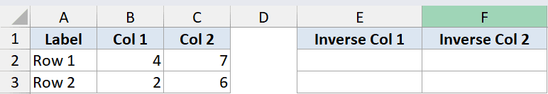
I want the inverse of this matrix to appear in the cells starting at E2.
Here is the formula:
=MINVERSE(B2:C3)
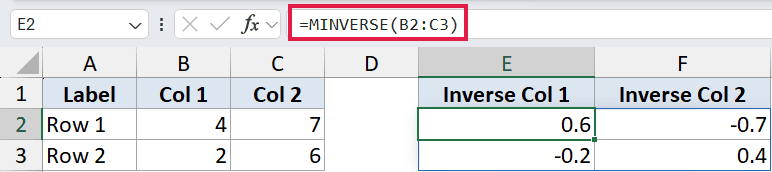
In Excel 365, you only enter the formula in cell E2. The result spills into E2:F3 on its own. You’ll see four numbers that are the inverse of the original matrix.
For the matrix [[4, 7], [2, 6]], the inverse comes out to roughly [[0.6, -0.7], [-0.2, 0.4]]. The determinant is 10, so dividing the cofactors by 10 gives those decimals.
Pro Tip: If you want to confirm the inverse is correct, multiply the original matrix by its inverse using MMULT. You should get the identity matrix back (1s on the diagonal, 0s everywhere else, give or take a few rounding crumbs). The formula is =MMULT(B2:C3, E2:F3).
Example 2: Invert a 3×3 Matrix
Now let’s bump up the size.
Below is the dataset. The range B2:D4 holds a 3×3 matrix. Same shape, just bigger.
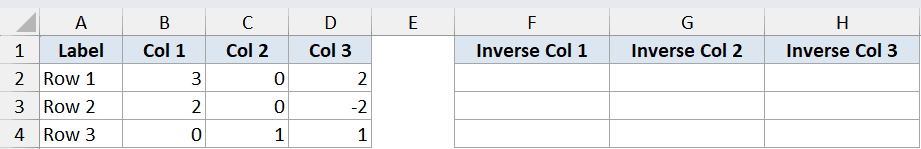
I want the inverse of this 3×3 matrix to spill into a 3×3 block starting at F2.
Here is the formula:
=MINVERSE(B2:D4)
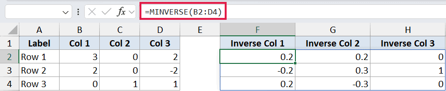
The formula goes in cell F2 only. The 9 inverse values spill across F2:H4.
In older versions of Excel (2019 and earlier), this won’t spill on its own. You’d have to select the F2:H4 range first, type the formula, and press Ctrl+Shift+Enter to lock it in as a legacy array formula.
You’ll know it worked because Excel wraps the formula in curly braces. In 365, none of that ceremony is needed.
Caveat: The numbers MINVERSE returns are computed to about 16 digits of precision. For most cases that’s plenty, but if you’re chaining inverses or doing repeated multiplications, tiny rounding errors can compound. Sanity-check the result against a known identity matrix when accuracy matters.
Example 3: Solve a 2-Equation System
Here’s where MINVERSE actually pays off.
Suppose you’re pricing two products. Two recent orders look like this:
- Order 1: 3 of Product A and 2 of Product B totaled $48
- Order 2: 1 of Product A and 4 of Product B totaled $46
(The numbers are made up, but they have a clean solution so you can verify it by hand.)
That’s two unknowns (the unit price of A and the unit price of B) and two equations. In matrix form, the coefficients go in a 2×2 matrix, and the order totals go in a 2×1 column.
Below is the dataset. B2:C3 holds the quantity matrix ([[3, 2], [1, 4]]) and E2:E3 holds the totals column ([[48], [46]]). The unknowns are the unit prices.
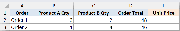
I want the unit prices of Product A and Product B to spill into G2:G3.
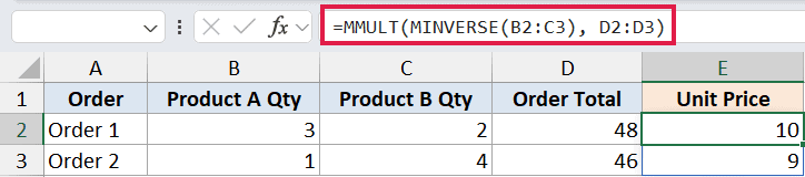
Here is the formula:
=MMULT(MINVERSE(B2:C3), E2:E3)
How this formula works:
MINVERSE(B2:C3)inverts the 2×2 coefficient matrix.MMULT(..., E2:E3)multiplies that inverse by the 2×1 totals column.- The result is a 2×1 column where each row is the unit price of the matching product.
You’ll see Product A at $10 and Product B at $9. You can verify by plugging the prices back in: 3×10 + 2×9 = 48, and 1×10 + 4×9 = 46.
The MMULT-of-MINVERSE pattern solves the whole system in a single spilled column.
Pro Tip: This is the matrix form of “x equals A inverse times b”. If you remember that pattern, you can solve any small linear system the same way. The trick is laying out the coefficient matrix and the right-hand side correctly. Each row in the matrix is one equation; the right-hand column holds the constants.
Example 4: Solve a 3-Equation System
Same idea, one size bigger.
Imagine a portfolio with three accounts. You know the totals after a year and you want to back out the starting balance in each account, given how the returns mixed.
Below is the dataset. B2:D4 is the 3×3 coefficient matrix, and F2:F4 is the column of right-hand-side values.
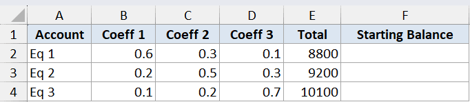
I want the three unknowns to spill down a single column starting at H2.
Here is the formula:
=MMULT(MINVERSE(B2:D4), F2:F4)
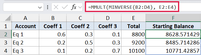
The combined formula does two things at once: inverts the 3×3, then multiplies the inverse by the 3×1 column. The 3 unknowns spill into H2:H4.
If the system has no unique solution (because the coefficient matrix is singular, meaning one equation is a linear combination of the others), MINVERSE will return #NUM! and the whole thing falls apart.
That’s actually useful information. It means the equations don’t have a unique answer, not that Excel did something wrong.
In older Excel versions, you’d select H2:H4 first, type the formula, and press Ctrl+Shift+Enter. In 365 you just type it in H2 and let it spill.
Example 5: Handle the Two Common Errors
Worth showing both errors deliberately so you recognize them on sight.
Below is the dataset. B2:C3 has a non-square issue (a blank cell or a text value in the range), and B5:C6 has a singular matrix (the second row is exactly double the first).
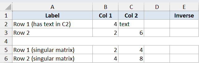
I want to deliberately trigger #VALUE! and #NUM! so you know what each one looks like and what’s actually broken.
Here are the formulas:
=MINVERSE(B2:C3)
=MINVERSE(B5:C6)
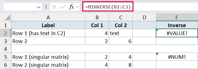
The first formula returns #VALUE!.
That happens when the input range isn’t a clean square of numbers. Common causes: a blank cell in the range, a text value, or a non-square shape (e.g., 2 rows by 3 columns).
The second formula returns #NUM!.
That happens when the matrix is square and all-numeric but mathematically non-invertible. The classic giveaway: one row is a scalar multiple of another, or the determinant is 0. You can check the determinant with =MDETERM(B5:C6). If it returns 0, MINVERSE won’t work on that matrix.
Caveat: There’s no IFERROR-style “give me a fallback inverse” for #NUM!. A singular matrix genuinely doesn’t have an inverse. The fix is to look at the data, not the formula. If two equations are essentially the same equation, the system itself is underdetermined.
Tips & Common Mistakes
- The matrix has to be square. Excel will not infer a square sub-region from a rectangular range. If you point MINVERSE at A1:C2, you get
#VALUE!, full stop. - Empty cells break it. A single blank cell anywhere in the range returns
#VALUE!. Same goes for text. Clean the range before calling MINVERSE. - In 365, just enter the formula in one cell. You no longer need to pre-select the output range and press Ctrl+Shift+Enter. The result spills automatically. If the spill range is blocked by existing values, you’ll see a #SPILL! error instead. Clear the cells below and the formula will land.
- In older Excel, CSE is mandatory. If you’re on Excel 2019 or earlier, you must select the output range first, type the formula, and press Ctrl+Shift+Enter. Forgetting CSE leaves just a single value in the top-left cell.
#NUM!means the matrix is singular. It is not a bug. The matrix you fed in genuinely has no inverse. Check the determinant with MDETERM. A determinant of 0 (or extremely close to 0) is the smoking gun.- Round-off is real. MINVERSE uses about 16-digit precision. Multiplying an inverse back into the original matrix should give the identity (the MUNIT function generates an identity matrix of any size), but expect a few values that are close to 1 or close to 0 rather than exactly 1 or 0.
- For large or sensitive matrix work, reach for a real tool. Excel handles small inversions (up to maybe 10×10 or so) just fine. For anything bigger, or for repeated chained operations, Python with NumPy or a dedicated stats package is more accurate and far easier to debug.
MINVERSE doesn’t come up every day, but the moment you have a small system to solve, it’s exactly the right tool.
The 2×2 and 3×3 cases cover most of the algebra people actually run into, and the MMULT pairing is the standard move for solving linear systems in a single formula.
If you want to take this further, look at MDETERM for checking invertibility up front, MUNIT for generating identity matrices to validate against, MMULT for chaining matrix operations together, and TRANSPOSE when you need to flip rows and columns before or after the inverse.
Related Excel Functions / Articles: