If you want to flip your data so rows become columns (or columns become rows), the TRANSPOSE function in Excel is one of the cleanest ways to do it.
TRANSPOSE is a native dynamic array function: in Excel 365 you type the formula in one cell, press Enter, and the transposed result spills across as many cells as the new shape needs.
In older versions (2019 and earlier) the same function exists but has to be entered as a CSE array formula. I’ll cover both, when to pick the formula over Paste Special, and a few practical patterns.
TRANSPOSE Function Syntax
Here is the syntax of the TRANSPOSE function:
=TRANSPOSE(array)
- array – The range of cells (or an array) you want to flip. Rows in this range become columns in the result, and columns become rows.
That’s the whole signature. One argument, and it’s the only one TRANSPOSE takes.
When to Use TRANSPOSE
Use this function when you need to:
- Flip a horizontal row of values into a vertical column (or the other way around)
- Keep the transposed result connected to the source so it updates when the source changes
- Pivot a small lookup table for use inside another formula (for example, inside SUMPRODUCT)
- Restructure data quickly for charts, reports, or layouts that simply read better the other way
Two Ways to Transpose Data in Excel
Before the examples, it helps to know there are really two paths to flipping rows and columns in Excel:
- The TRANSPOSE function – returns a live, linked output that updates whenever the source data changes. Spills automatically in Excel 365.
- Paste Special > Transpose – a one-time copy that creates a static, disconnected snapshot.
If you need the output to stay in sync with the source, use the TRANSPOSE function.
If you just want a quick one-off flip and don’t care about future updates, Paste Special is faster.
The rest of this article focuses on the function. For the keyboard shortcut version, see our guide on transposing data in Excel with shortcuts, and for a side-by-side view of every method, the broader walkthrough on how to convert columns to rows in Excel is a good companion.
Let me show you a few practical examples of how to use TRANSPOSE.
Example 1: Spill a Column Into a Row in Excel 365
Let’s start with a simple example.
Below is a column of tour cities in A2:A8 (seven stops on a small concert tour) that I want to flip into a single horizontal row for a poster layout.

Here is the formula:
=TRANSPOSE(A2:A8)
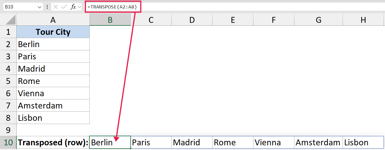
In Excel 365, you type the formula in one cell, hit Enter, and the transposed output spills across as many cells as the source has rows. No selecting the destination range first, no Ctrl+Shift+Enter.
The blue spill border around the output is Excel telling you the formula is the source for that whole range.
Edit the formula in the top-left cell to change everything. The rest of the cells are read-only spill outputs.
Pro tip: If you change a value in A2:A8, the transposed row updates instantly because TRANSPOSE returns a live reference, not a copy.
Example 2: Use Legacy CSE TRANSPOSE in Older Excel
Here’s how the same job works in older versions of Excel (2019 and earlier) where dynamic arrays don’t exist.
Same column of seven tour cities in A2:A8. The goal is identical: flip it into a horizontal row.
Here is the formula:
=TRANSPOSE(A2:A8)
The formula text is the same, but the entry method is not.
In legacy Excel you have to:
- First, select the output range that matches the transposed shape. For a 7-row column you’d select 7 cells in a single row.
- Type the formula
=TRANSPOSE(A2:A8)into the active cell of that selection. - Press Ctrl+Shift+Enter (CSE) instead of just Enter.
Excel wraps the formula in curly braces {=TRANSPOSE(A2:A8)} and treats it as a single array formula filling the whole selection.
If you press just Enter by mistake, you’ll only see the first value (or a #VALUE! error). Re-select the range, click into the formula bar, and press Ctrl+Shift+Enter to fix it.
Caveat: Legacy array formulas cannot be edited cell-by-cell. To change anything, select the entire output range first, then edit and re-confirm with Ctrl+Shift+Enter. In Excel 365 you don’t have to think about any of this, the formula just spills.
Example 3: Spill a Two-Dimensional Range
Now let’s look at something a bit more interesting.
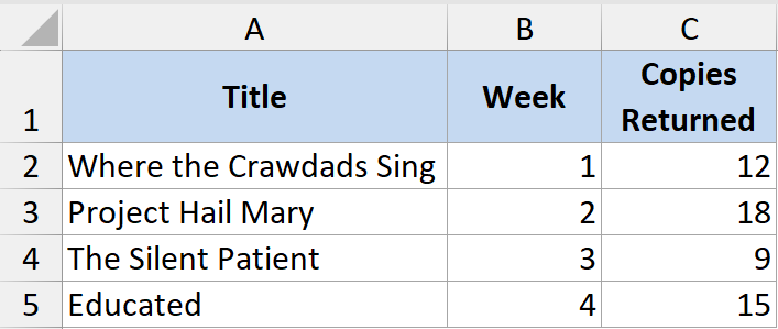
Below is a small library checkout table in A1:C5 with the book title, week, and number of copies returned. I want to flip it so the headers run down the side instead of across the top.
Here is the formula (entered in cell E1 in Excel 365):
=TRANSPOSE(A1:C5)
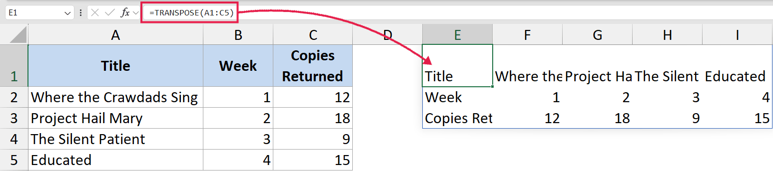
In the above formula, TRANSPOSE takes the 5-row by 3-column range and spills a 3-row by 5-column range.
The first row of the source (the headers) becomes the first column of the output, the second row becomes the second column, and so on.
This is the most common real-world use: pivoting a table sideways for a report layout, a chart, or just to make a wide table fit better on screen.
Because TRANSPOSE spills natively in 365, you don’t have to pre-select the destination block. Pick a single anchor cell and Excel sizes the spill for you.
Example 4: Linked Output vs Static Copy
Let me show you why people pick the TRANSPOSE function over Paste Special.
Same column of seven tour cities in A2:A8. I’ll do it both ways, then change one of the source values.
The formula version:
=TRANSPOSE(A2:A8)
The Paste Special version: copy A2:A8, right-click an empty cell, choose Paste Special, tick “Transpose”, click OK.
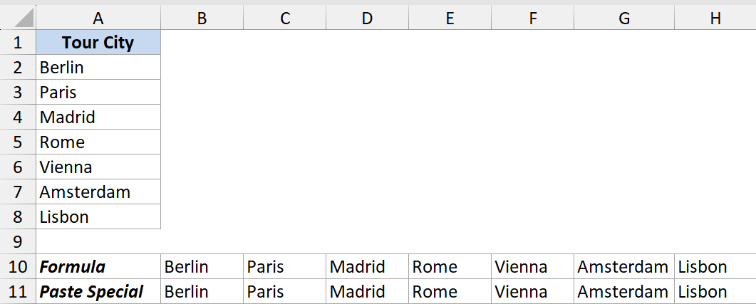
Both look identical at first.
But if you change “Berlin” to “Hamburg” in A4, the formula output updates automatically. The Paste Special output stays as “Berlin” because it was copied as a static value.
Use the formula whenever the source might change. Use Paste Special when you want a frozen snapshot you can edit independently.
Tips & Common Mistakes
- It spills in Excel 365. TRANSPOSE is a native dynamic array function, so in 365 / 2021 / Web you enter it in one cell and the transposed result spills automatically. No CSE, no pre-selecting the destination range.
- #SPILL! error in Excel 365. This means something is blocking the spill range. Clear the cells where the result needs to land, and the formula will populate them automatically.
- Watch for the
@implicit intersection. If a workbook is saved by older Excel, modern Excel sometimes auto-injects an@symbol (for example,=@TRANSPOSE(...)). That collapses the spill to a single cell. Remove the@and the rotated output comes back. - #VALUE! error in older Excel. In 2019 or earlier, this usually means you forgot Ctrl+Shift+Enter, or you selected the wrong number of cells before entering the formula. Make sure your output selection matches the transposed shape (rows of source = columns of output, and vice versa) and re-confirm with CSE.
- CSE is obsolete in 365. If you’re on 365 / 2021 / Web, you do NOT need Ctrl+Shift+Enter. Pressing just Enter is correct, and the formula spills.
- TRANSPOSE keeps the data type. Numbers stay numbers, dates stay dates, formulas inside the source range get evaluated. You can’t use TRANSPOSE to convert text to numbers.
- It returns a reference, not a copy. Any change in the source ripples into the transposed output. If you want a static snapshot instead, copy the TRANSPOSE result and Paste Special as Values.
- Size limits exist but rarely matter. Legacy CSE transpose tops out around 5,461 elements. In Excel 365 the practical limit is your worksheet size, so this is almost never an issue today.
- You can nest TRANSPOSE inside other formulas. For example,
=SUMPRODUCT(TRANSPOSE(A2:A8), B2:B8)lets you multiply a row by a column without rearranging your data first. It also pairs well with TEXTSPLIT for jobs like splitting text to rows in Excel. - Need to flip a whole table, not just a column? The same TRANSPOSE logic applies, and there are a few extra tricks worth knowing if you want to flip data in Excel end-to-end.
That covers how the TRANSPOSE function works, when to reach for it instead of Paste Special, and how to handle it in both Excel 365 and older versions.
The function itself is dead simple. The only part that trips people up is the dynamic-array versus CSE entry method, and once you know which version of Excel you’re on, that decision is automatic.
Related Excel Functions / Articles:
- SORT Function in Excel
- How to Transpose Multiple Rows into One Column in Excel
- Row vs Column in Excel – What’s the Difference?
- Microsoft Excel Terminology (Glossary)
- How to Swap Columns in Excel?
- SPILL Error in Excel – How to Fix?
- How to Swap Cells in Excel (3 Easy Ways)
- Bulk Find and Replace in Excel