SIGN Function in Excel

The SIGN function in Excel returns 1 for a positive number, -1 for a negative number, and 0 for zero.

It is useful when the direction of a change matters more than its size. You can use the result in comparisons, labels, or directional adjustments.

In this article, I’ll show you how to classify positive and negative values, label differences from a plan, and apply adjustments based on direction.

SIGN Function Syntax in Excel

The SIGN function needs one number or numeric expression.

=SIGN(number)

• number is required. It can be any real number or a formula that returns one.

SIGN returns 1 for a positive number, 0 for zero, and -1 for a negative number.

When to Use SIGN Function

• Classify values as positive, negative, or zero.
• Compare actual results with planned values.
• Turn numeric differences into readable status labels.
• Apply a separate adjustment amount in the right direction.

Example 1: Classify Positive, Negative, or Zero

Let’s start with a simple service queue report.

Below is the dataset with each service queue and its weekly change.

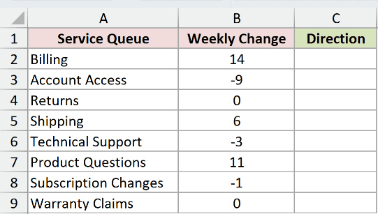
I want to return 1 for an increase, -1 for a decrease, and 0 when the queue did not change.

Here is the formula:

=SIGN(B2:B9)

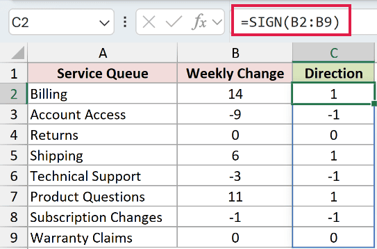
The range in column B goes into SIGN as one array. Excel places the eight results in cells C2:C9.

Billing has a positive change of 14, so SIGN returns 1. Account Access has -9, so it returns -1. Returns has zero, so it returns 0.

Pro Tip: Keep cells C2:C9 empty before entering the formula. Any value in that destination range will block the spill and produce a #SPILL! error.

Example 2: Compare Actual and Planned Values

Here’s a practical way to classify performance against a plan.

Below is the dataset with planned and completed field visits for eight offices.

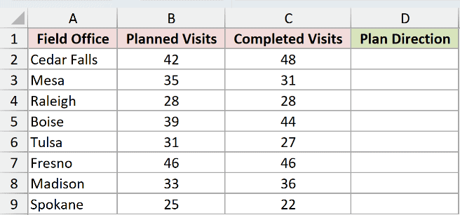
I want to identify which offices finished above plan, below plan, or exactly on plan.

Here is the formula:

=SIGN(C2:C9-B2:B9)

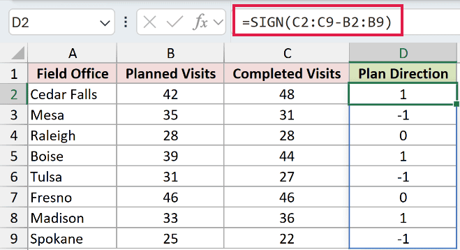
Excel first subtracts the planned visits in column B from the completed visits in column C. SIGN then classifies each difference.

The results are 1, -1, 0, 1, -1, 0, 1, and -1. A 1 means above plan, while -1 means below plan.

Zero means the planned and completed numbers match.

Example 3: Convert SIGN Results to Status Labels

Numeric codes are useful in calculations, but text labels are often easier to read in a report.

Below is the dataset with target and actual output for eight production lines.

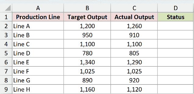
I want to label each production line as Below Target, On Target, or Above Target.

Here is the formula:

=CHOOSE(SIGN(C2:C9-B2:B9)+2,"Below Target","On Target","Above Target")

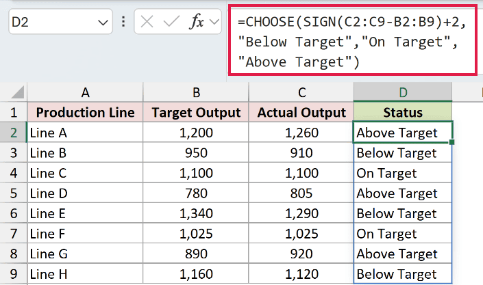
How this formula works:

• C2:C9-B2:B9 calculates the difference between actual and target output.
• SIGN converts each difference to -1, 0, or 1.
• Adding 2 changes those codes to 1, 2, or 3.
• CHOOSE uses those numbers to return Below Target, On Target, or Above Target.

The formula returns Above Target, Below Target, On Target, Above Target, Below Target, On Target, Above Target, and Below Target.

If you only need the labels, IFS is a more direct option in Excel 2019 and later.

Use =IFS(C2:C9>B2:B9,"Above Target",C2:C9<B2:B9,"Below Target",TRUE,"On Target").

The SIGN and CHOOSE version is handy when you also want to reuse the -1, 0, and 1 direction codes elsewhere.

Example 4: Apply Directional Adjustments

SIGN can also apply the direction from one column to a separate magnitude in another column.

Below is the dataset with adjustment minutes and moisture shortfall readings for eight irrigation zones.

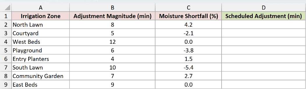
I want positive shortfalls to add minutes, negative shortfalls to remove minutes, and zero to make no adjustment.

Here is the formula:

=B2:B9*SIGN(C2:C9)

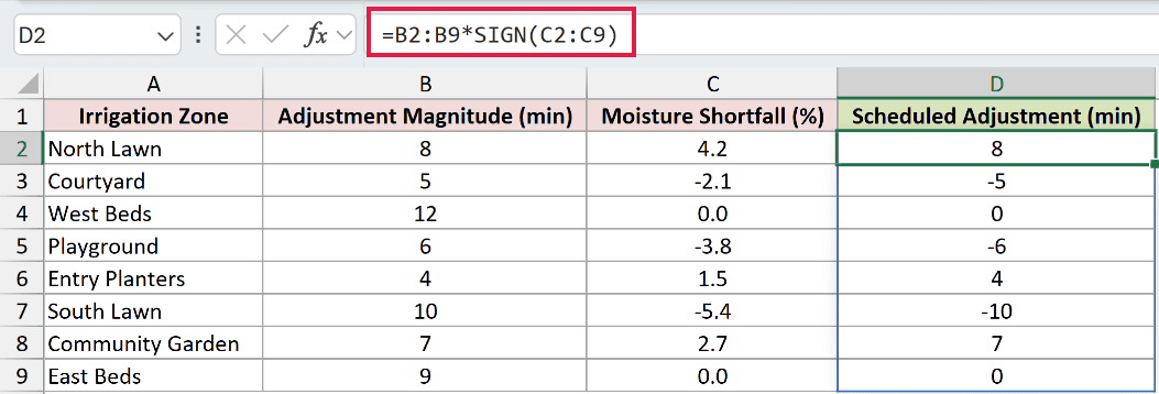
SIGN reads the direction from the moisture shortfall in column C. Excel multiplies that code by the adjustment magnitude in column B.

The scheduled adjustments are 8, -5, 0, -6, 4, -10, 7, and 0 minutes.

The magnitude stays separate from the measurement that decides the direction. This makes the formula easy to audit and update.

Pro Tip: Use ABS when you need a number’s positive magnitude. Multiplying a number by its own SIGN result also makes it positive, but =ABS(number) is clearer.

Tips & Common Mistakes

• SIGN returns numeric codes. It does not return text such as “Positive” or “Negative.”
• Text that Excel cannot treat as a number produces a #VALUE! error.
• In Excel 2021 and later, a range formula spills automatically. Excel 2019 and earlier needs a copied formula or a legacy array formula.
• Do not add the @ operator before SIGN when you want multiple results. It reduces a range calculation to one value through implicit intersection.
• If you want to remove a negative sign and keep the magnitude, use ABS instead of SIGN.

I covered how SIGN classifies numbers, compares values, creates status labels, and applies directional adjustments.

I hope you found this article helpful.

List of All Excel Functions