
The CHOOSE function in Excel returns an item from a list of values using a position number, starting at one.
You can map a WEEKDAY result to a label or let RANDBETWEEN select an item. CHOOSE can also rearrange references for a VLOOKUP formula.
In this article, I’ll show you how to convert indexes into labels, assign letter grades, and build a left lookup with VLOOKUP.
CHOOSE Function Syntax in Excel
The CHOOSE function returns a value from a list of values based on its position number.
=CHOOSE(index_num, value1, [value2], ...)
Where:
- index_num: the position of the value you want to return. Must be between 1 and 254.
- value1: the first value in the list. Required.
- value2, value3, …: additional values, up to 254 total. Optional.
The values can be text, numbers, cell references, ranges, or even nested formulas.
When to Use CHOOSE Function
A few common scenarios:
- Pick a value from a fixed list by its position (e.g., department name from a code).
- Map a number to a label (e.g., 1-7 to day names, 1-12 to month names or fiscal quarters).
- Convert scores or ranks into letter grades or category labels without nested IFs.
- Randomly select an option from a predefined list when combined with RANDBETWEEN.
- Rearrange columns inside a lookup function so VLOOKUP can pull values from the left.
Example 1: Basic CHOOSE Syntax
Let’s start with the simplest possible example.
Below is a small parameter card with the Department Index in B1 and a placeholder for the Department name in B2.
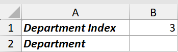
I want to return the department name that corresponds to the index in B1.
Here is the formula:
=CHOOSE(B1, "Marketing", "Sales", "Engineering", "Finance", "HR")

CHOOSE reads the value in B1 (which is 3) and returns the 3rd value from the list, which is “Engineering”. Change B1 to any number from 1 to 5 and the result updates instantly.
Example 2: Spill Department Names from a Column of Indexes
Now let’s see what CHOOSE does when you feed it a range of indexes in Excel 365.
Below is a list of 8 employees, each with a department index in column B (1 through 5).
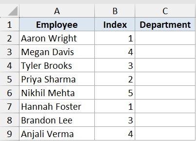
I want to fill the entire Department column with the actual department name for each employee, using a single formula.
Here is the formula:
=CHOOSE(B2:B9, "Marketing", "Sales", "Engineering", "Finance", "HR")
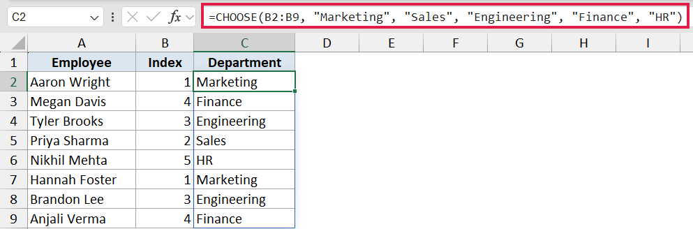
CHOOSE takes the array of indexes in B2:B9 and returns the matching department name for each row. The result spills down from C2 to C9 without any need to fill the formula down manually.
Pro Tip: In older Excel versions that don’t support dynamic arrays, the same formula would need to be entered with Ctrl+Shift+Enter (as a CSE array), or you’d have to write a per-row formula and fill it down for each employee.
Example 3: Return a Day Name Using CHOOSE + WEEKDAY
Here’s a classic use of CHOOSE. Turning a date into a custom day-of-week label.
Below is a list of 8 order dates in column A, and an empty Day column in column B.
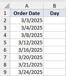
I want to show a 3-letter day abbreviation (Sun through Sat) next to each order date.
Here is the formula:
=CHOOSE(WEEKDAY(A2:A9), "Sun", "Mon", "Tue", "Wed", "Thu", "Fri", "Sat")
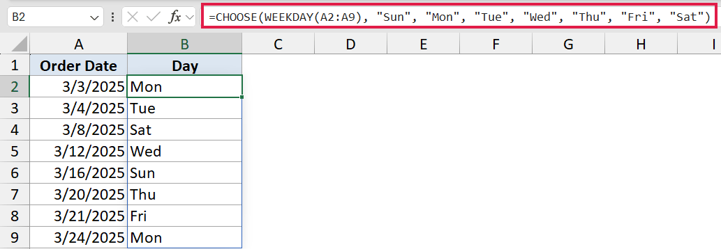
WEEKDAY returns a number from 1 (Sunday) to 7 (Saturday) for each date in the range. CHOOSE then picks the matching day abbreviation from the list, and the whole thing spills down column B.
In Excel 365, you could also do this with =TEXT(A2:A9, "ddd"), which returns Sun/Mon/Tue directly. For more standard approaches, see our full guide on how to convert a date to a day of the week. The CHOOSE version wins when you want custom labels (like “Weekday” / “Weekend”, or labels in another language) instead of the standard abbreviations.
Example 4: Convert Scores into Letter Grades
Here’s a clever way to use CHOOSE to replace a long nested IF with a single, much cleaner formula.
Below is a list of 8 students with their exam scores in column B.
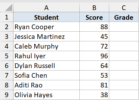
I want to assign a letter grade based on the score. F for under 51, C for 51-70, B for 71-90, and A for 91 and above.
Here is the formula:
=CHOOSE((B2:B9>=0)+(B2:B9>=51)+(B2:B9>=71)+(B2:B9>=91), "F", "C", "B", "A")
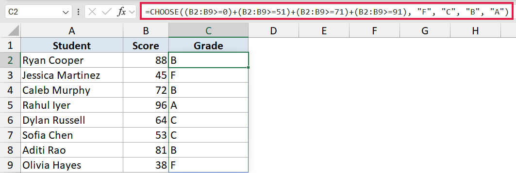
Each (score >= threshold) comparison returns TRUE (1) or FALSE (0). Adding the four results gives a number from 1 to 4, which is perfect input for CHOOSE.
How this formula works:
- A score of 88 → (1) + (1) + (1) + (0) = 3 → CHOOSE returns “B”
- A score of 45 → (1) + (0) + (0) + (0) = 1 → “F”
- A score of 96 → (1) + (1) + (1) + (1) = 4 → “A”
The whole formula spills down the Grade column in one shot.
In Excel 2019 and 365, the SWITCH and IFS functions handle this kind of bucketing more directly. But this CHOOSE pattern still works in any version of Excel and stays much shorter than a nested IF chain.
Example 5: Random Team Assignment Using CHOOSE + RANDBETWEEN
If you want to pick a random value from a fixed list, CHOOSE works well with RANDBETWEEN.
Below is a list of 8 participants in column A and an empty Team column in column B.
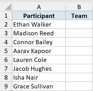
I want to roll a random team for each participant. Either Red, Blue, or Green.
Here is the formula:
=CHOOSE(RANDBETWEEN(1,3), "Red", "Blue", "Green")
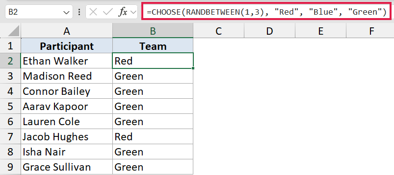
RANDBETWEEN generates a random integer between 1 and 3, and CHOOSE picks the matching team color. The formula is filled down so each row rolls its own number independently.
Pro Tip: RANDBETWEEN is volatile, which means the random team will reshuffle every time the worksheet recalculates. Once you’ve assigned everyone, lock the result by copying column B and pasting it back as values (Paste Special → Values).
Example 6: Left Lookup Using CHOOSE + VLOOKUP
VLOOKUP normally can’t return a value from a column to the left of the lookup column. The CHOOSE + VLOOKUP combo works around that.
Below is a small employee table with Name in column A and Employee ID in column B (the wrong order for a normal VLOOKUP). Right below the table is a small lookup card where I’ve typed an Employee ID in B10.
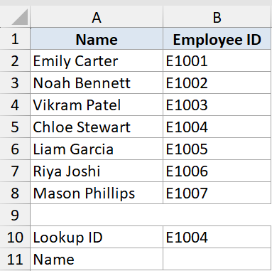
I want to look up the employee name for ID “E1004”, even though Name sits to the left of the ID column.
Here is the formula:
=VLOOKUP(B10, CHOOSE({1,2}, B2:B8, A2:A8), 2, FALSE)
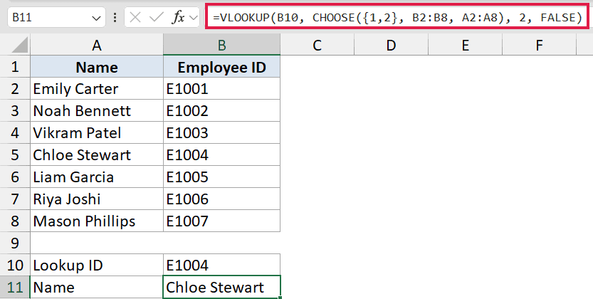
The CHOOSE({1,2}, B2:B8, A2:A8) part builds a virtual 2-column array on the fly, with Employee ID as column 1 and Name as column 2. VLOOKUP then searches column 1 for “E1004” and returns the matching name from column 2, which is “Chloe Stewart”.
In Excel 365, XLOOKUP is the modern replacement for this trick. =XLOOKUP(B10, B2:B8, A2:A8) does the same thing in one clean step, without the CHOOSE workaround. The CHOOSE + VLOOKUP pattern is still worth knowing if you’re sharing the file with someone on an older version of Excel.
Tips & Common Mistakes
- #VALUE! error on out-of-range index: CHOOSE returns the #VALUE! error if the index_num is less than 1 or larger than the number of values you supplied. Wrap the index in IFERROR, or clamp it with MAX and MIN, to keep the formula from breaking.
- 254-value hard limit: CHOOSE only accepts up to 254 value arguments. For a longer mapping, switch to a lookup-based approach (VLOOKUP, XLOOKUP, INDEX + MATCH) with a reference table.
- Modern alternatives: For specific-value matching (e.g., status code to label), SWITCH and IFS in Excel 2019 and 365 are usually cleaner than CHOOSE. For picking entire rows or columns from an array, use CHOOSEROWS and CHOOSECOLS in Excel 365.
- Fractional indexes are truncated: An index of 2.7 is treated as 2, not rounded to 3. Wrap it in ROUND if you want the nearest whole number.
- In Excel 365, CHOOSE spills: Feeding a range of indexes makes CHOOSE return an array that spills down or across. Make sure the cells in the spill range are empty, otherwise you’ll get a #SPILL! error.
CHOOSE looks basic on its own, but it gets a lot more useful when you pair it with WEEKDAY, RANDBETWEEN, VLOOKUP, or boolean arithmetic. In Excel 365, feeding it a range of indexes makes it spill the whole result in one formula.
Newer functions like SWITCH, XLOOKUP, and CHOOSEROWS handle some of these jobs more directly. CHOOSE is still worth knowing because it works in every version of Excel and keeps the formula short.
Related Excel Functions / Articles:
- MATCH Function in Excel
- LOOKUP Function in Excel
- SEQUENCE Function in Excel
- OFFSET Function in Excel
- XLOOKUP Vs INDEX MATCH in Excel
- Microsoft Excel Terminology (Glossary)
- Bulk Find and Replace in Excel
- Using VLOOKUP Approximate Match in Excel (Examples)
- INDEX Function in Excel
- How to Use VLOOKUP with Multiple Criteria in Excel
