
Excel’s TRIMMEAN function returns an average after excluding a specified proportion of values from the high and low ends of a dataset.
It removes the same number of values from each end, then averages what remains. This reduces the influence of extreme observations.
The percentage controls the total excluded from both ends. You can use FILTER first when the trimmed average should cover only a selected group.
In this article, I’ll show you how to calculate a trimmed mean, compare trimming percentages, and apply the calculation to a filtered group.
TRIMMEAN Function Syntax in Excel
The TRIMMEAN function has two required arguments:
=TRIMMEAN(array, percent)
arrayis the array or range of values you want to trim and average.percentis the fraction of all data points to exclude. Excel splits the exclusions equally between the top and bottom of the dataset.
Excel rounds the number of excluded data points down to the nearest multiple of two. That rule keeps the trimming balanced between both ends.
When to Use TRIMMEAN Function
- Calculate an average that is less affected by unusually high or low values.
- Compare results at several trim percentages.
- Apply the same percentage-based trimming rule across repeated reports.
- Find a trimmed mean for records that meet a condition.
Example 1: Calculate a 20% Trimmed Mean
We’ll start with a set of 12 calibration readings.
Below is the dataset with the calibration run IDs and their readings.
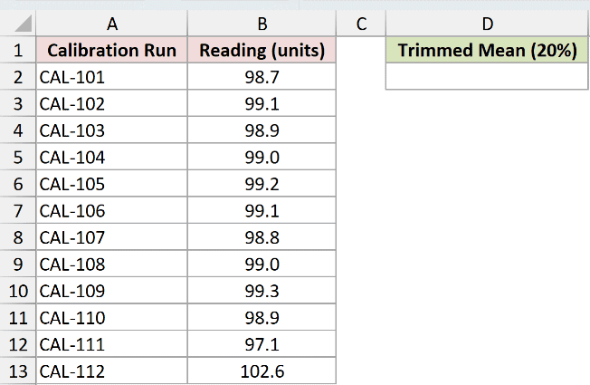
I want to exclude 20% of the readings and average the values left in the middle.
Here is the formula:
=TRIMMEAN(B2:B13,20%)
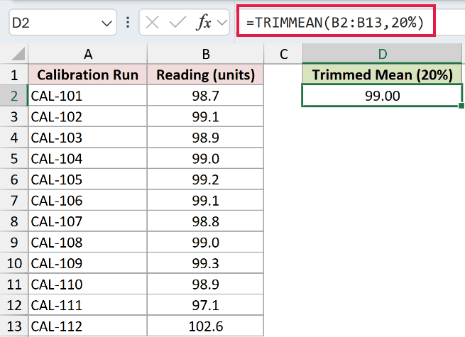
The range contains 12 readings. Twenty percent of 12 is 2.4, which Excel rounds down to two excluded values.
It removes 97.1 and 102.6, one from each end. The mean of the remaining 10 readings is 99.00.
Pro Tip: The percentage covers both tails together. A 20% trim removes 10% from the low end and 10% from the high end when the count permits it.
Example 2: How TRIMMEAN Rounds Odd Counts
This example shows what happens when the requested percentage produces an odd number of exclusions.
Below are 10 calibration readings, including one much higher value.
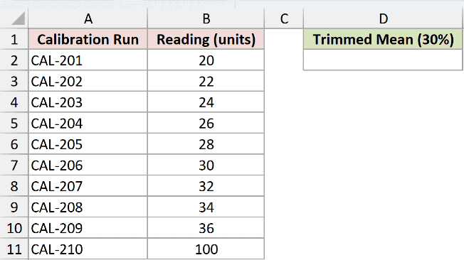
I want to request a 30% trim and see how many readings Excel actually excludes.
Here is the formula:
=TRIMMEAN(B2:B11,30%)
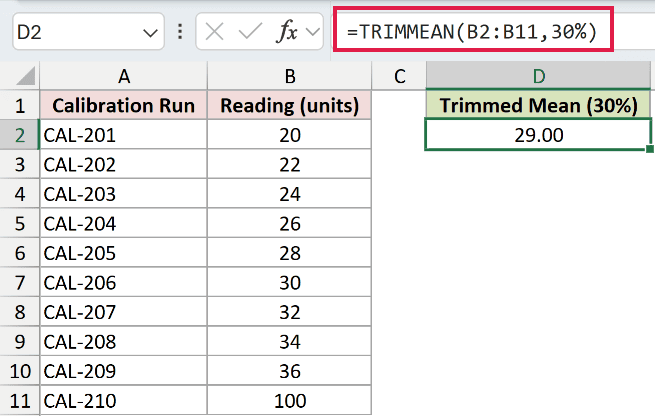
Thirty percent of 10 is three. Excel needs an even number for balanced trimming, so it rounds three down to two.
The function removes 20 and 100. The remaining eight readings average to 29.00.
Pro Tip: Multiply the number of numeric values by the trim percentage, then round down to the nearest even whole number. That is the total number Excel excludes.
Example 3: Compare Several Trim Percentages
You can also compare several percentages against the same readings.
Below is a dataset of 20 readings and a small comparison table for 0%, 10%, 20%, and 40% trims.
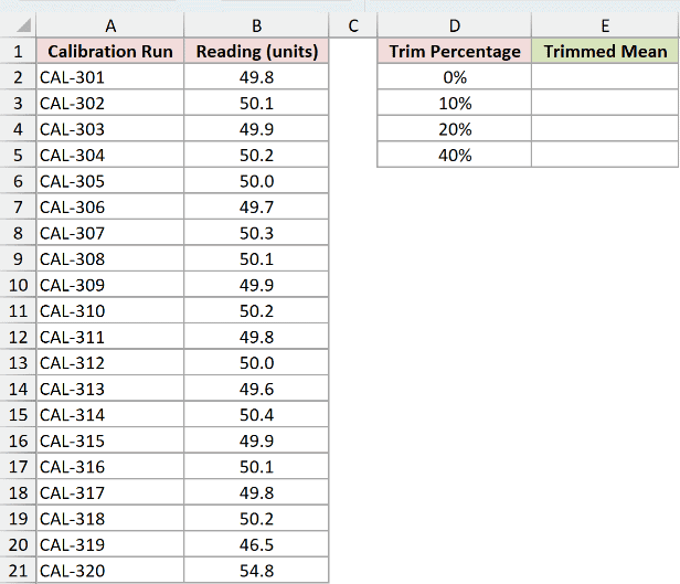
I want each row in the comparison table to use the percentage beside it.
Enter this formula in cell E2 and copy it down through E5:
=TRIMMEAN($B$2:$B$21,D2)
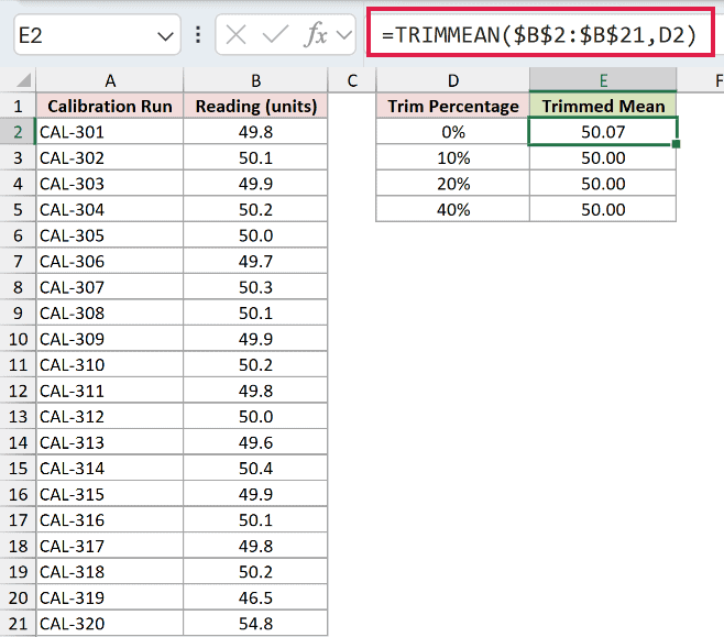
The absolute reference keeps the readings fixed as the formula moves down. The reference to D2 changes to D3, D4, and D5.
With no trimming, the mean is 50.07 when displayed to two decimals. The 10%, 20%, and 40% trimmed means each display as 50.00.
The equal results are specific to these readings. Other datasets can produce a different mean at each trim level.
Example 4: Conditional TRIMMEAN with FILTER
Suppose you only want to average the calibration runs marked Priority.
Below is the dataset with the run ID, priority status, and reading.
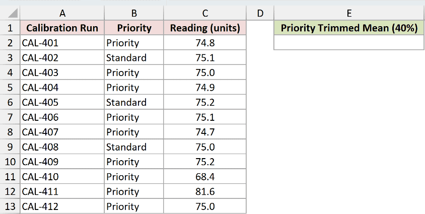
I want to filter the Priority readings first, then calculate their 40% trimmed mean.
Here is the formula:
=TRIMMEAN(FILTER(C2:C13,B2:B13="Priority"),40%)
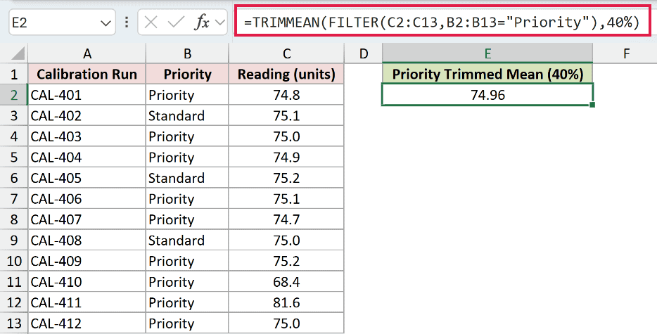
FILTER returns the nine Priority readings. TRIMMEAN then excludes 68.4 and 81.6 before averaging the remaining seven values.
The final trimmed mean is 74.96 when displayed to two decimal places.
Pro Tip: FILTER is available in Excel 2021, Excel 2024, and Microsoft 365. In an older version, filter or copy the matching records to a separate range first.
Tips & Common Mistakes
- Treat
percentas the total fraction removed from both ends, not the fraction removed from each end. - Expect Excel to round the requested number of exclusions down to the nearest even whole number.
- A negative
percentor a value above 1 returns a#NUM!error. - Remember that TRIMMEAN returns one value. It does not spill the remaining records into the worksheet.
- Check whether an unusual value is an error before excluding it. A valid extreme value may still matter to your analysis.
I covered a basic trimmed mean, Excel’s even-count rounding, percentage comparisons, and a conditional calculation with FILTER.
I hope you found this article helpful.
Other Excel articles you may also like:
