
Excel’s AVERAGE function returns the arithmetic mean of a set of numbers.
It adds the numeric values and divides by their count. Zeros count toward the average, while empty cells and text in referenced ranges are ignored.
In this article, I’ll show you how to calculate row averages, handle zeros, and average the top values or a filtered subset.
AVERAGE Function Syntax in Excel
The AVERAGE function takes one or more numbers, cell references, or ranges and returns their arithmetic mean.
=AVERAGE(number1, [number2], ...)
- number1 (required): The first number, cell reference, or range you want to average.
- number2, … (optional): Up to 254 additional numbers, references, or ranges. You can mix and match them in the same formula.
When to Use AVERAGE Function
- Calculating the average sales across a set of months, weeks, or quarters.
- Finding a student’s average score across multiple tests.
- Tracking average response times or any operational metric you measure repeatedly.
- Combining numbers from non-adjacent ranges into a single average.
- Feeding the result of a FILTER or other dynamic array formula into a conditional average.
Example 1: Average of a Single Column
Let’s start with the most common use of AVERAGE. You have a column of numbers and you want a single average.
Below is the dataset. Column A lists the months from January to December, and column B has the monthly sales figures for the year.
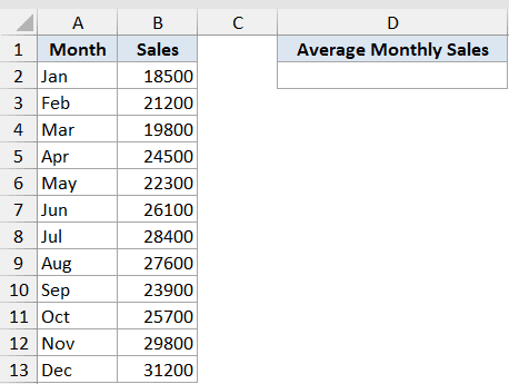
We want to find the average monthly sales for the whole year.
Here is the formula:
=AVERAGE(B2:B13)
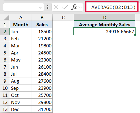
AVERAGE adds up the 12 sales values in B2:B13 and divides the total by 12. The result is about 24,917, which is what the average monthly sales worked out to across the year.
This is the pattern you’ll use 90% of the time. One range in, one number out.
Example 2: Average Across Multiple Ranges
AVERAGE doesn’t have to take a single contiguous range. You can pass it several ranges separated by commas, and it treats them all as one big pool of numbers.
Below is the dataset. There are 8 weeks of sales for Product A in column B and Product B in column C.
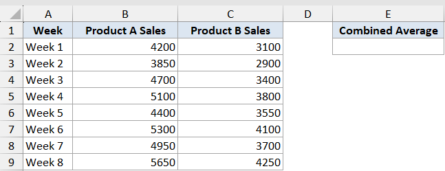
We want the combined average across both products, treating every weekly figure as one entry.
Here is the formula:
=AVERAGE(B2:B9, C2:C9)
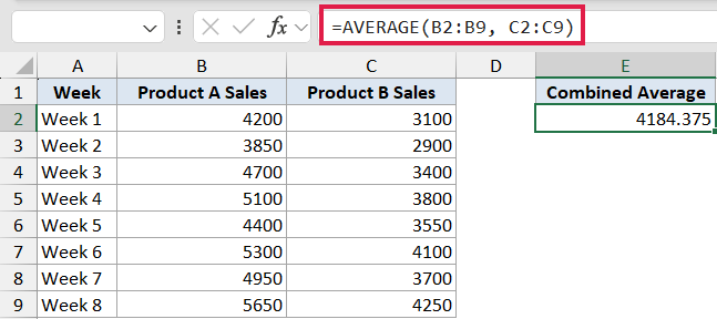
This pulls in all 16 values (8 weeks × 2 products) and gives back a single average of about 4,184.
You can keep adding ranges separated by commas, up to 255 arguments. The ranges don’t have to be the same shape or size either.
This is handy when your data sits in non-adjacent blocks and you don’t want to copy it all into one column just to average it.
Example 3: Average Score Per Student (Per-Row Average)
When your data is laid out so each row is a separate “thing” (a student, a sales rep, a product), you usually want one average per row rather than one average for the whole table.
Below is the dataset. Each row is a student, with their scores across four tests sitting in columns B through E.
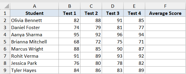
We want each student’s average score in column F.
Here is the formula:
=AVERAGE(B2:E2)
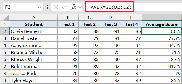
Enter the formula in F2 and drag it down to F9. As you copy it down, the row references shift, so F3 calculates the average of B3:E3, F4 averages B4:E4, and so on.
The result is one average per student. Olivia comes in at 86.5, Aanya at 94.25, Tyler at 85.5, and so on across the eight students.
Example 4: AVERAGE Includes Zeros, AVERAGEIF Excludes Them
This one trips a lot of people up. AVERAGE ignores blank cells and cells containing text, but it does include zeros as valid numbers. If your zeros mean “no data” rather than “actually zero,” your average will be lower than you expect.
Below is the dataset. Each row is a day of the week, and column B has the number of minutes exercised that day. The 0s in days 3, 6, and 9 are rest days.
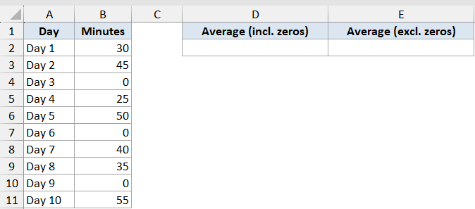
We want to see both averages side by side: one that counts the rest days as 0 minutes, and one that ignores them entirely.
Here are the two formulas:
=AVERAGE(B2:B11)
=AVERAGEIF(B2:B11,"<>0")
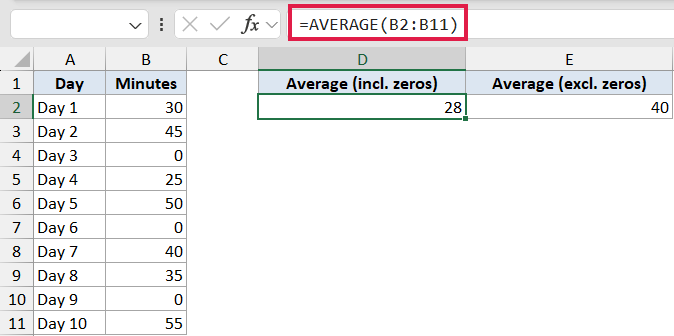
The first formula gives you 28 minutes per day. It averages all 10 days, including the three zeros.
The second one gives you 40 minutes per day. The "<>0" criterion (using Excel’s does not equal operator) tells AVERAGEIF to skip any cell whose value is zero.
Which one is correct depends entirely on what the zeros mean in your data. If a rest day is genuinely “zero minutes of exercise,” the 28 is the honest number. If “no data recorded” got entered as 0 instead of left blank, the 40 is closer to the truth.
Pro Tip: Blank cells, text, and logical values like TRUE/FALSE are always skipped by AVERAGE. Only zeros need the AVERAGEIF workaround. If your “missing” entries are blanks (not zeros), plain AVERAGE already does what you want.
Example 5: Average of the Top 3 Values
Sometimes you don’t want the average of everything. You just want the average of the top few performers, and to skip the rest.
Below is the dataset. Column A has 10 sales reps and column B has their sales for the period.
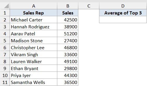
We want the average sales of just the top 3 reps.
Here is the formula:
=AVERAGE(LARGE(B2:B11,{1,2,3}))
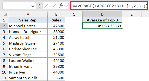
How this formula works:
LARGE(B2:B11, {1,2,3})pulls back the 1st, 2nd, and 3rd largest values from the range. The{1,2,3}is an array constant that asks for all three positions in one shot.AVERAGE(...)then takes those three numbers and averages them.
The result is about 49,033, which is the mean of the top three sales numbers (51,200, 49,100, and 46,800).
To average the bottom 3 instead, swap LARGE for SMALL: =AVERAGE(SMALL(B2:B11,{1,2,3})). To average the top 5, change the array constant to {1,2,3,4,5}.
Example 6: AVERAGE Inside FILTER (Conditional Average)
In Excel 365, you can pair AVERAGE with FILTER to average only the rows that match a condition. This is the modern replacement for many AVERAGEIF patterns and it scales naturally to more complex criteria.
Below is the dataset. Each row is an order, with the order ID in column A, the region in column B, and the sale amount in column C.
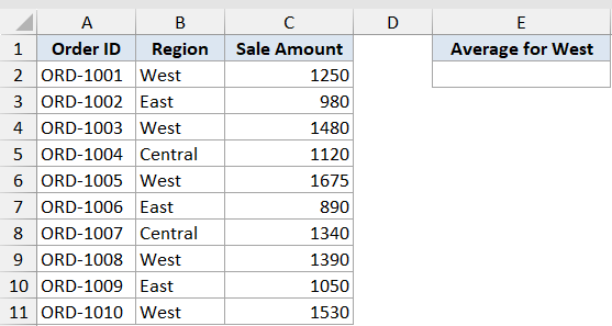
We want the average sale amount, but only for orders from the West region.
Here is the formula:
=AVERAGE(FILTER(C2:C11,B2:B11="West"))
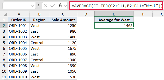
How this formula works:
FILTER(C2:C11, B2:B11="West")returns just the sale amounts where the region is “West.” In this dataset, that’s five orders.AVERAGE(...)then averages those five values, giving you 1,465.
You can do the same job with =AVERAGEIF(B2:B11,"West",C2:C11), and for one simple condition that’s still fine.
But the FILTER version pulls ahead as soon as you need more flexible criteria. You can combine conditions with * for AND and + for OR, and chain other functions onto the filtered output.
For example, =AVERAGE(FILTER(C2:C11, (B2:B11="West")*(C2:C11>1300))) averages only the West orders above 1,300.
Tips & Common Mistakes
- Zeros get counted, blanks don’t. This is the single most common AVERAGE confusion. If your “no data” cells are 0s, they pull the average down. Either replace them with blanks or use AVERAGEIF with
"<>0". - Error values break the formula. If any cell in your range contains an error like
#N/Aor#DIV/0!, the AVERAGE formula will return an error too. Wrap the range in IFERROR, or use=AGGREGATE(1, 6, range)which has a built-in “ignore errors” mode. - Numbers stored as text are ignored. If a column looks numeric but the values are actually text (left-aligned by default, often imported from a CSV), AVERAGE will silently skip them. A quick way to check is to use COUNT on the range. If it returns fewer than expected, you have text-looking numbers.
- Empty ranges return #DIV/0!. If every cell in your range is blank or text, AVERAGE has nothing to divide by. Guard against it with
=IF(COUNT(C2:C11)>0, AVERAGE(C2:C11), ""). - Use AVERAGEA when text and TRUE/FALSE should count. AVERAGEA treats TRUE as 1, FALSE as 0, and text as 0. It rarely gives you what you want, but it’s there if you need it.
AVERAGE is one of those functions that looks simple until you actually use it on messy data. Knowing how it handles zeros, blanks, and errors saves a lot of “why is my average wrong” debugging later.
For conditional work, AVERAGEIF and AVERAGEIFS are the next stop, or you can wrap AVERAGE around FILTER for the dynamic array version. And when each value should count for more than the others, the weighted average formula is what you actually want.
Related Excel Functions / Articles:
- SUMPRODUCT Function in Excel
- SUBTOTAL Function in Excel
- Calculate the Population Mean in Excel
- Microsoft Excel Terminology (Glossary)
- Mean Median Mode Calculator
- How to Sum a Column in Excel?
- How to Calculate Variance in Excel?
- How to Calculate Standard Deviation in Excel?
- SUM Function in Excel
- Calculate Average Percentage in Excel
