
Excel’s NUMBERVALUE function converts text to a number using the decimal and grouping separators you specify.
That is useful for imported amounts whose separators differ from your regional settings. You can tell Excel how to read the text before using it in totals.
The result is numeric; its display format is a separate choice.
In this article, I’ll show you how to convert imported numbers with different separators, handle percentage text, and fix amounts that will not sum.
NUMBERVALUE Function Syntax in Excel
NUMBERVALUE takes the text to convert, followed by two optional separator arguments:
=NUMBERVALUE(text, [decimal_separator], [group_separator])
- text (required) is the text you want to convert into a number. You can supply a cell reference or, in Excel 2021 and later, a range.
- decimal_separator (optional) is the character separating the whole-number part from the decimal part. Put a literal character in double quotes. If omitted, Excel uses your current locale’s decimal separator.
- group_separator (optional) is the character separating groups of digits, usually thousands. If omitted, Excel uses your current locale’s group separator.
The separator arguments describe the source text. They don’t set how the resulting numbers look; the result cells’ number format controls that.
NUMBERVALUE is available in Excel 2013 and later. The range formulas below need Excel 2021 or later to spill automatically.
When to Use NUMBERVALUE Function
- Convert imported amounts that use different decimal and thousands separators from your Excel settings.
- Turn percentages stored as text into numeric rates you can calculate with.
- Read exports that use an unusual grouping character, such as an apostrophe.
- Convert a text column before totaling it with SUM.
- Handle imported number formats that VALUE can’t interpret using your current locale.
Example 1: Convert European-Format Numbers to Real Numbers
Let’s start with a supplier price list that uses commas for decimals and periods for thousands.
Below is the dataset. Column A contains product codes, and B2:B9 contains list prices stored as text, including 1.234,56 and 987,05.
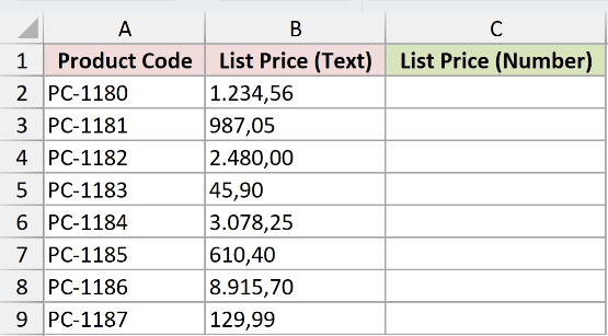
We want to convert all eight prices into numbers with one formula.
Here is the formula to enter in C2:
=NUMBERVALUE(B2:B9,",",".")
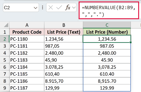
The results spill into C2:C9. The second argument tells Excel to read the comma as the decimal separator, while the third identifies the grouping period.
For product PC-1180, 1.234,56 becomes 1,234.56 in C2. The next price, 987,05, becomes 987.05 in C3.
A grouping period doesn’t need to appear in every input. Excel can still convert the smaller prices using the same formula.
Column C uses the number format #,##0.00, so each converted price displays two decimal places.
Pro Tip: Choose separators by looking at the imported text, not at how you want the answer displayed. Here, "," means the source uses decimal commas.
Example 2: Convert Percentages Stored as Text
Now let’s convert rates that already use the workbook’s expected decimal separator.
Below is the dataset. Column A lists loan products, and B2:B9 holds percentage text such as 3.5%, 7%, and 4.875%.
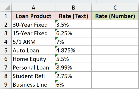
We want numeric percentages that can be used in calculations.
Here is the formula to enter in C2:
=NUMBERVALUE(B2:B9)
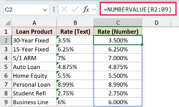
This time, both separator arguments are omitted. Excel uses the current locale’s separators, which match the period decimals in this example.
NUMBERVALUE recognizes the trailing percent sign and divides the numeric part by 100. You don’t need to divide the result again.
The formula spills into C2:C9. With the 0.000% format applied, C2 displays 3.500%, C4 displays 7.000%, and C5 displays 4.875%.
The extra decimal places come from the number format. The conversion is what makes these rates usable as numbers.
Pro Tip: Omitting the separators makes this formula depend on your locale. For imported text with different separators, specify them explicitly as in Example 1.
Example 3: Use Custom Separators From an Export
Some exports use an apostrophe to group thousands, so commas and periods aren’t the only characters you’ll encounter.
Below is the dataset. Column A contains part numbers, and B2:B9 holds text costs using period decimals and apostrophe grouping, such as 2'845.60.
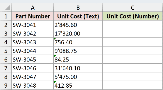
We want to convert the costs without manually removing the apostrophes.
Here is the formula to enter in C2:
=NUMBERVALUE(B2:B9,".","'")
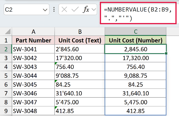
The second argument identifies the decimal period. The third argument contains an apostrophe enclosed in double quotes, telling Excel which grouping character to ignore.
The formula spills into C2:C9. The first cost displays as 2,845.60, and the second displays as 17,320.00.
The text 756.40 in B4 becomes the number displayed as 756.40 in C4. The appearance stays the same, but the cell now holds a usable number.
You can name a custom separator directly instead of adding a separate text-cleaning formula.
Example 4: Fix Imported Text That Won’t SUM
Here’s where converting text makes a visible difference to a total.
Below is the dataset. Column A lists branches, and B2:B9 contains Q1 revenue stored as text, with decimal commas and spaces between digit groups.
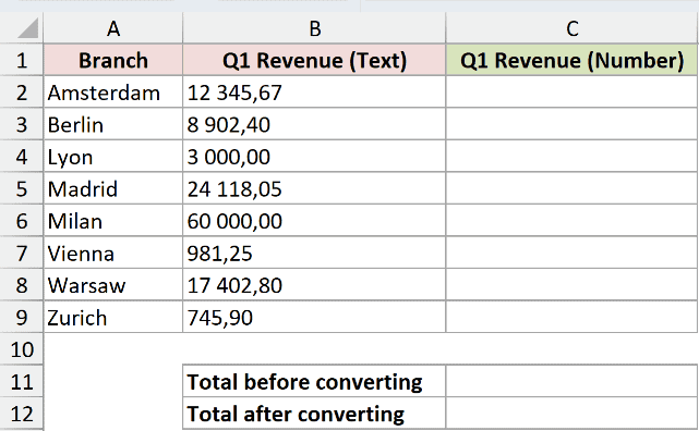
We want to convert the revenue and compare totals before and after conversion.
Here is the conversion formula to enter in C2:
=NUMBERVALUE(B2:B9,","," ")
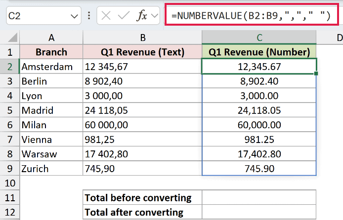
The formula spills into C2:C9. Amsterdam’s 12 345,67 becomes 12,345.67, and Berlin’s 8 902,40 becomes 8,902.40.
The comma argument tells Excel where the decimals begin. NUMBERVALUE ignores spaces automatically, before interpreting separators, so the third argument does no extra work here.
Here is the total of the original text column, entered in C11:
=SUM(B2:B9)
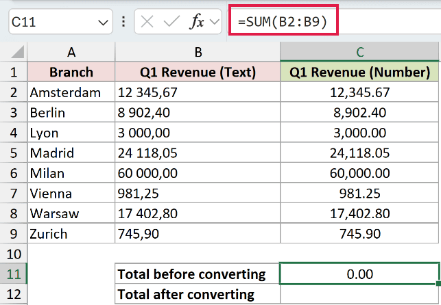
C11 displays 0.00. SUM ignores the text values in the referenced range, even though they look like revenue amounts.
And here is the total of the converted numbers, entered in C12:
=SUM(C2:C9)
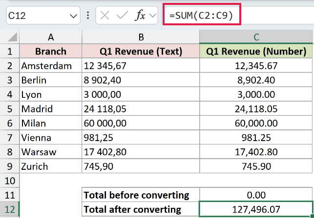
C12 displays 127,496.07. The two totals sit below the dataset, with the original total in C11 and the converted total directly beneath it.
The difference between the two totals shows you that the converted column now holds numbers SUM can add.
Pro Tip: If the same import arrives every week, consider Power Query’s Transform > Data Type > Using Locale conversion. You can reuse that import step, while NUMBERVALUE remains useful for conversions directly on the worksheet.
Example 5: NUMBERVALUE vs VALUE on Imported Amounts
Let’s compare the two functions on exactly the same source text.
Below is the dataset. Column A contains transaction IDs, and B2:B9 contains amounts stored as text with decimal commas and period grouping.
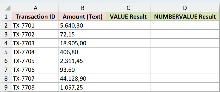
We want to see how each function handles separators that don’t match the workbook’s locale.
Here is the VALUE formula to enter in C2:
=VALUE(B2:B9)
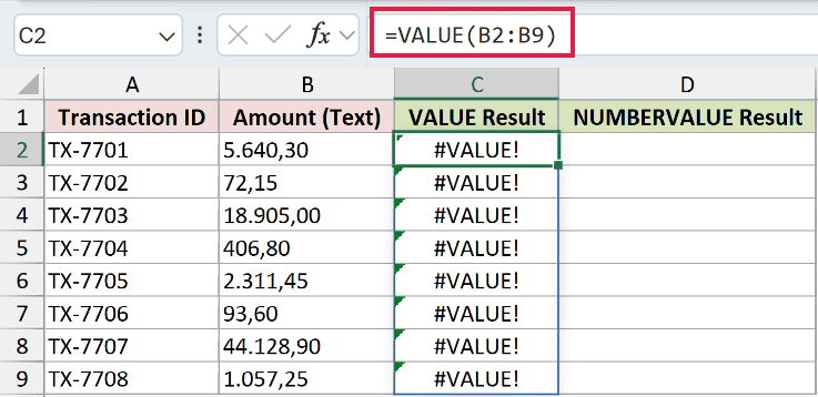
Every cell in C2:C9 returns #VALUE! in this workbook. These errors are intentional: VALUE can’t interpret these amounts using the current locale.
VALUE has no arguments for specifying different decimal or grouping characters.
Here is the NUMBERVALUE formula to enter in D2:
=NUMBERVALUE(B2:B9,",",".")
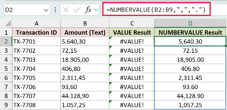
The results spill into D2:D9, and every amount converts successfully. D2 displays 5,640.30, D3 displays 72.15, and D4 displays 18,905.00.
The difference is explicit separator handling. NUMBERVALUE reads the comma as the decimal separator and the period as the grouping separator.
VALUE is still useful when the source text already matches your locale. Its errors here don’t mean it fails on European-format text in every Excel setup.
NUMBERVALUE has no Microsoft 365-era successor to switch to. When you need control over the source separators, this is the function to use.
Tips & Common Mistakes
- Name the source separators in the correct order. The decimal separator comes second, and the group separator comes third. Those settings describe the input text, not the desired display format.
- Keep the output cells clear. In Excel 2021 and later, these range formulas spill automatically. An occupied output cell can cause
#SPILL!, and an implicit-intersection@can reduce an array result to one value. - Use one cell and fill down in older versions. In Excel 2013 through Excel 2019, reference the first input cell instead of the full range, then copy the formula down. The spill examples don’t require Ctrl+Shift+Enter in Excel 2021 and later.
- Check malformed source text. A decimal separator appearing twice, or a group separator appearing after the decimal separator, causes
#VALUE!. Fix the source text or incorrect separator arguments. - Use one character per separator. If you supply several characters, NUMBERVALUE uses only the first. A longer string doesn’t define several alternative separators.
- Watch percentage signs. Each trailing percent sign applies another division by 100. An accidental extra sign changes the numeric rate.
- Consider Text to Columns for a one-off conversion. Its Advanced settings let you specify decimal and thousands separators without keeping a formula column.
Start by checking which characters the source uses, then pass those separators to NUMBERVALUE.
For imported amounts, comparing SUM before and after conversion gives you a useful check that the values are ready for calculations.
