FIXED Function in Excel

Excel’s FIXED function rounds a number to a specified number of decimal places, adds optional thousands separators, and returns the formatted result as text.

That text return is the main distinction. A cell number format changes appearance while keeping the value numeric, but FIXED changes its underlying type.

I’ll show you the default output, negative decimal settings, text labels, and an explicit conversion back to numbers for a SUM calculation.

FIXED Function Syntax in Excel

The syntax of the FIXED function is:

=FIXED(number, [decimals], [no_commas])

• number is the numeric value you want to round and convert to text.
• [decimals] is the number of digits to the right of the decimal point. It defaults to 2.
• A negative [decimals] value rounds to the left of the decimal point.
• [no_commas] is TRUE to remove thousands separators. FALSE or omission keeps them.

When to Use FIXED Function

• Create text with a consistent number of decimal places.
• Include or remove thousands separators in exported text.
• Round values to tens, hundreds, or thousands before converting them to text.
• Combine formatted numbers with labels, identifiers, or units.
• Prepare a text number for explicit conversion with VALUE.

Example 1: Default Decimals and No Commas

We’ll begin with the two most common FIXED settings.

Below is the dataset with six project estimates and empty columns for the default output and a version without thousands separators.

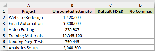
I want one text column with the default formatting and another without commas.

Here is the default formula entered in C2, spilling through C7:

=FIXED(B2:B7)

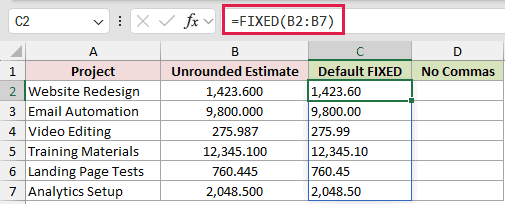
Because [decimals] is omitted, FIXED uses two decimal places. The first result is 1,423.60, and 275.987 rounds to 275.99.

Now I can suppress the thousands separators while keeping two decimal places.

Here is the no-commas formula entered in D2, spilling through D7:

=FIXED(B2:B7,2,TRUE)

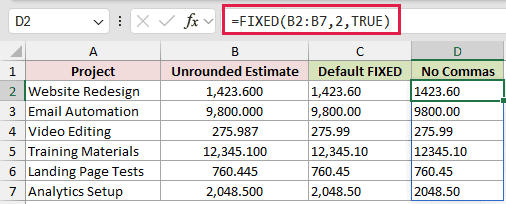
The first result becomes 1423.60 instead of 1,423.60. Both results are text, regardless of whether the comma appears.

Pro Tip: These range formulas spill in Excel 2021, Excel 2024, and Microsoft 365. In Excel 2019 and earlier, use a single-cell formula and fill it down.

Example 2: Round With Negative Decimals

Negative decimal arguments move the rounding position to the left of the decimal point.

Below is the budget-adjustment dataset with positive and negative values, plus empty text columns for tens, hundreds, and thousands.

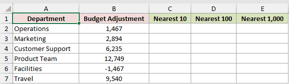
I want to compare the same adjustments rounded to three different positions.

Here is the nearest-10 formula entered in C2, spilling through C7:

=FIXED(B2:B7,-1)

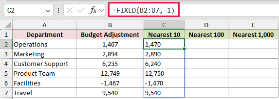
The formula rounds 1,467 to 1,470, 2,894 to 2,890, and -1,467 to -1,470.

Here is the nearest-100 formula entered in D2, spilling through D7:

=FIXED(B2:B7,-2)

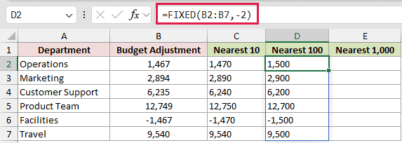
With -2, those values become 1,500, 2,900, and -1,500.

Here is the nearest-1,000 formula entered in E2, spilling through E7:

=FIXED(B2:B7,-3)

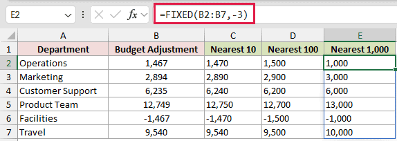
With -3, the same values become 1,000, 3,000, and -1,000. The final column still contains text, even though every result looks numeric.

Use the ROUND function instead when you need the rounded result to remain a number.

Example 3: Add a Number to a Text Label

FIXED is useful when the final result is meant to be read as text.

Below is the shipment dataset with measured lengths and an empty column for customer labels.

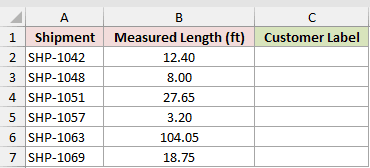
I want each label to combine the shipment ID, a one-decimal length, and the ft unit.

Here is the label formula entered in C2, spilling through C7:

=A2:A7&" | "&FIXED(B2:B7,1)&" ft"

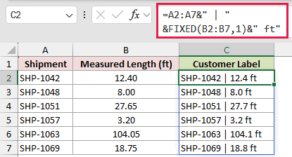
FIXED formats each length with one decimal place. The ampersands join that text to the matching shipment ID and unit.

The results include SHP-1042 | 12.4 ft, SHP-1048 | 8.0 ft, and SHP-1063 | 104.1 ft.

For currency, dates, percentages, or custom patterns, the TEXT function offers more formatting control.

Example 4: Convert FIXED Text Before SUM

This example makes the text-versus-number difference visible in a calculation.

Below is the four-column invoice dataset: Invoice, Source Amount, FIXED Text, and Converted Number. Two empty total cells sit below the table.

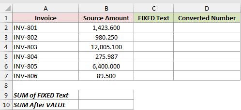
I want to compare SUM on the FIXED text with SUM after an explicit numeric conversion.

Here is the FIXED formula entered in C2, spilling through C7:

=FIXED(B2:B7,2)

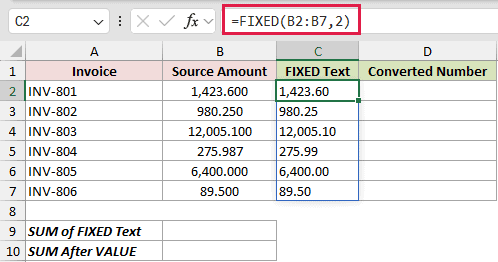
The formula creates six text values with two decimal places. For example, 1,423.600 becomes the text 1,423.60.

Next, I can convert that text column back to numbers deliberately.

Here is the conversion formula entered in D2, spilling through D7:

=VALUE(C2:C7)

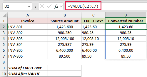
The VALUE function converts each recognized numeric text string into a numeric value. Column D can then use normal number formatting.

Now I can test the original FIXED text column with SUM.

Here is the first total formula entered in B9:

=SUM(C2:C7)

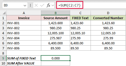
The formula returns 0 because SUM ignores text values stored in referenced cells.

Here is the converted-number total formula entered in B10:

=SUM(D2:D7)

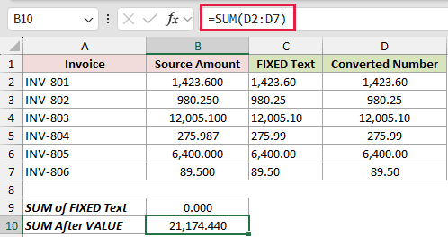
After conversion, SUM returns 21,174.44.

Excel can coerce recognized numeric text in some arithmetic formulas, so VALUE is not required for every operator. Here, it creates an explicitly numeric column before SUM.

Pro Tip: If calculation is the next step, keep the source numeric and apply a cell number format. Use FIXED when the text result itself is required.

Tips & Common Mistakes

• FIXED returns text. Applying another number format to that result does not convert it back to a number.
• The default is two decimal places. Supply [decimals] when you need a different number of digits.
• Set no_commas to TRUE when an export or identifier must not contain thousands separators.
• Negative decimals round to the left of the decimal point. They do not create decimal digits.
• Excel numbers support at most 15 significant digits. FIXED cannot restore precision that the source number does not contain.
• Separators can follow Excel’s regional settings. The screenshots use a period for decimals and a comma for thousands.

I covered default formatting, comma suppression, negative decimal rounding, text labels, and numeric conversion with FIXED.

I hope you found this article helpful.

List of All Excel Functions

Related Excel Functions / Articles:

• How to Round to the Nearest Whole Number in Excel
• How to Round Numbers in Excel Without Formula?
• ROUNDDOWN Function in Excel