
If imported data has blank rows or columns around its edges, TRIMRANGE can return a smaller rectangular array containing the populated cells.
TRIMRANGE is available in Excel for Microsoft 365. Its result spills, so keep the required output area empty.
In this article, I’ll show you how to remove blank outer rows and columns, preserve interior blanks, and trim a range before sorting it.
TRIMRANGE Function Syntax in Excel
The TRIMRANGE function accepts a range or array, followed by optional settings for rows and columns.
=TRIMRANGE(range,[trim_rows],[trim_cols])
- range is the range or array you want to trim.
- trim_rows controls which blank outer rows are removed. Use 0 for none, 1 for leading, 2 for trailing, or 3 for both.
- trim_cols applies the same four choices to blank outer columns.
If you omit both optional arguments, Excel uses 3 for each. That removes blank rows and columns from both outer edges.
TRIMRANGE stops scanning an edge when it reaches a nonblank cell. It keeps blank rows, columns, and cells that sit inside the remaining rectangle.
When to Use TRIMRANGE Function
- Remove blank outer rows and columns from imported data.
- Keep leading blanks while removing trailing blanks, or do the reverse.
- Give another dynamic array function a range whose boundary follows the data.
- Build a full-column list that expands and contracts with its populated cells.
- Use a trim reference when the same direction should apply to both rows and columns.
Example 1: Remove Blank Rows and Columns from Both Edges
We’ll begin with TRIMRANGE’s default behavior.
Below is a lab import inside A2:E8. The actual table occupies B3:D7, with blank rows and columns around it.
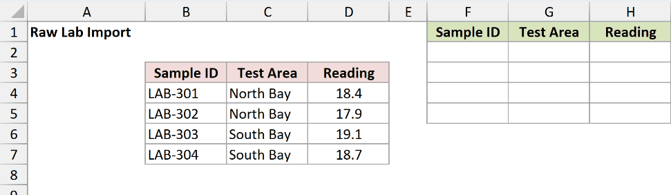
I want to return only the populated table.
Here is the formula in F1:
=TRIMRANGE(A2:E8)
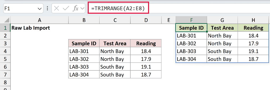
Because both optional arguments are omitted, TRIMRANGE removes blank rows and columns from both edges.
The result spills into F1:H5. It includes the header and four lab records, from LAB-301 through LAB-304.
Pro Tip: TRIMRANGE changes the returned boundary. It does not delete, move, or edit the source cells.
Example 2: Remove Leading Blank Rows and Both Blank Columns
The row and column settings can use different trim directions.
Below is an archive import in A2:E8. Row 2 is blank, rows 7 and 8 are trailing blanks, and columns A and E are blank.
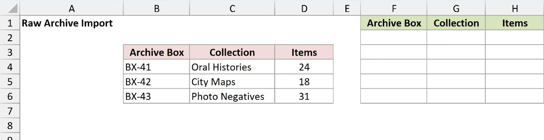
I want to remove only the leading blank row while trimming blank columns from both sides.
Here is the formula in F1:
=TRIMRANGE(A2:E8,1,3)
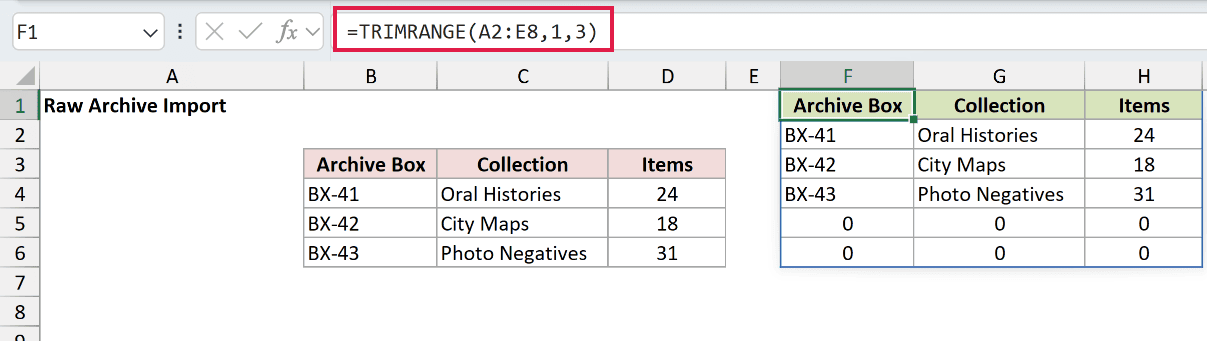
The 1 trims leading blank rows. The 3 trims leading and trailing blank columns.
Excel returns B3:D8, so the three archive records remain above two blank rows. In a direct spilled reference, those retained blank cells display as zeros.
This distinction matters. A blank inside the returned rectangle is preserved, even when its displayed spill value looks like zero.
Example 3: Remove Trailing Blank Rows and Both Blank Columns
This example reverses the row direction.
Below is a translation import in A2:E9. The header starts in row 2, and rows 7 through 9 are blank.
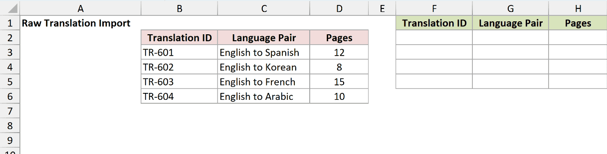
I want to keep the leading row and remove the trailing blank rows.
Here is the formula in F1:
=TRIMRANGE(A2:E9,2,3)
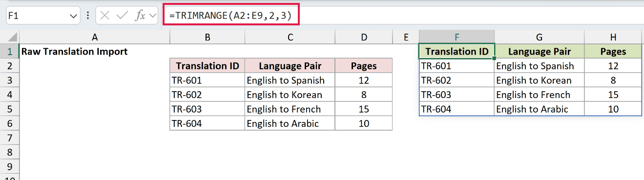
The 2 removes trailing blank rows, while the 3 removes blank columns from both outer edges.
The result is B2:D6, returned in F1:H5. It contains the header and all four translation records.
Example 4: Keep an Interior Blank Row
TRIMRANGE removes blank outer edges, not blank records inside the data.
Below is a reservation list with a completely blank fourth row between two groups of bookings.
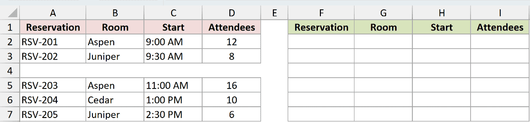
I want to see what the default formula returns when the blank row sits inside the range.
Here is the formula in F1:
=TRIMRANGE(A1:D7)
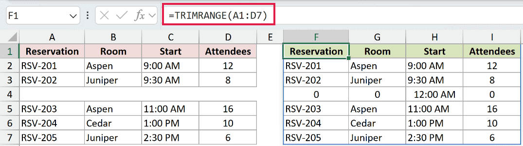
The first and last rows already contain data, so there is nothing to remove from those edges.
The result keeps row 4. Its referenced blanks display as zeros, with the time-formatted blank displaying as 12:00 AM.
Use FILTER when you need to remove records by a condition. TRIMRANGE only adjusts the outer boundary.
Pro Tip: Check the source for interior blanks before using the result. TRIMRANGE will not close gaps that appear between populated rows or columns.
Example 5: Trim a Range Before Sorting It
TRIMRANGE can prepare an array for another function.
Below is a permit import in A3:E9. The records occupy B3:D7, with blank outer rows and columns.
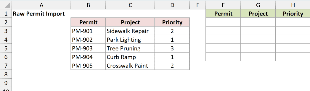
I want to trim the import and sort the five records by Priority in ascending order.
Here is the formula in F2:
=SORT(TRIMRANGE(A3:E9),3,1)
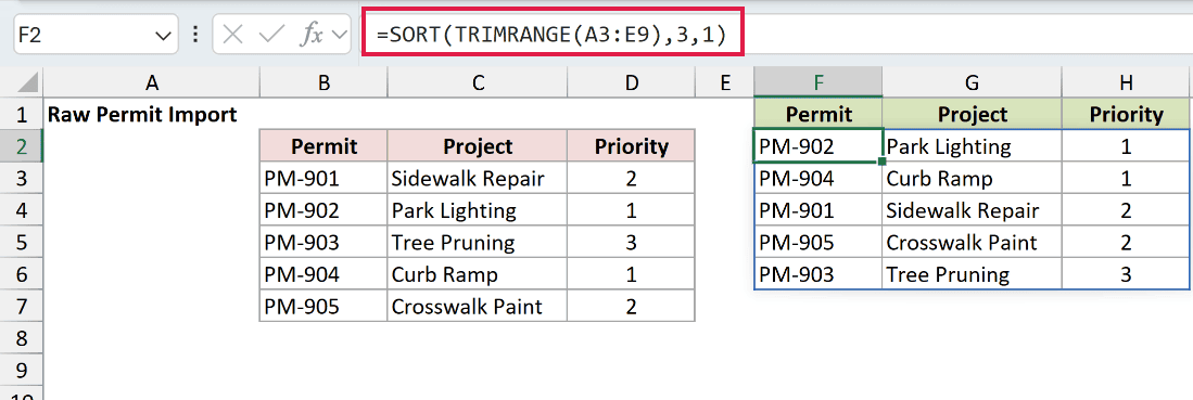
TRIMRANGE first returns B3:D7. The SORT function then uses the third returned column and ascending order.
PM-902 and PM-904, both with Priority 1, appear first. Priority 2 follows, and PM-903 with Priority 3 appears last.
Example 6: Create a Dynamic List from a Full Column
TRIMRANGE also accepts full-column references.
Below is a workshop list in column A. The heading is in A1, five workshop names follow, and the rest of the column is blank.
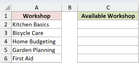
I want a spilled list of the workshop names without the heading.
Here is the formula in C2:
=DROP(TRIMRANGE(A:A),1)
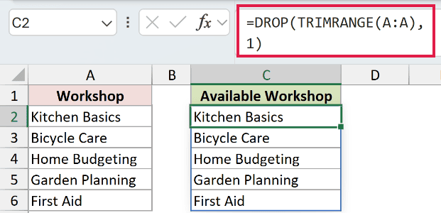
TRIMRANGE shortens A:A to its populated section, A1:A6. The DROP function then removes the first returned row.
The five workshop names spill through C6. Adding another name directly below the source list expands the trimmed range and the returned list.
Pro Tip: An Excel Table is often easier for a normal entered-data list. TRIMRANGE is useful when you must work with a range or array.
Example 7: Use Trim References as Shorthand
Excel provides three trim reference operators for common TRIMRANGE settings.
Below is a single-column range, A2:A8. It has one leading blank, four numbers, and two trailing blanks.
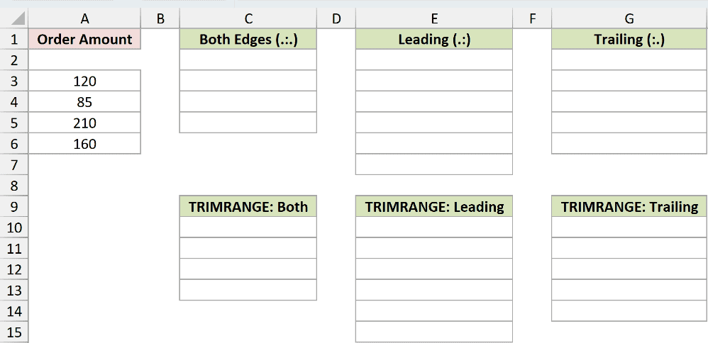
I want to compare each operator with its equivalent TRIMRANGE formula.
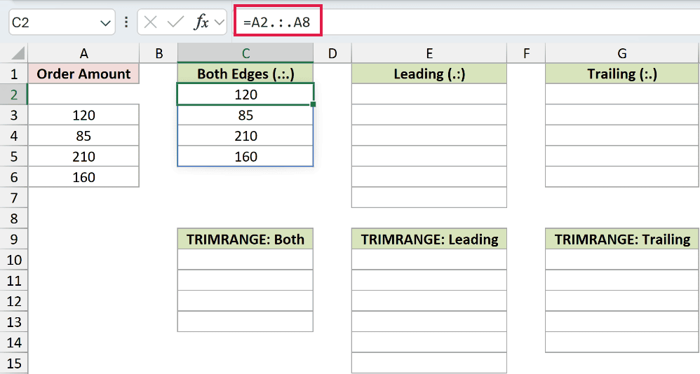
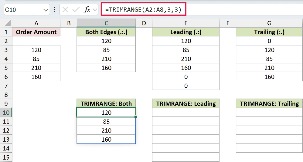
The .:. operator trims both leading and trailing blanks:
=A2.:.A8
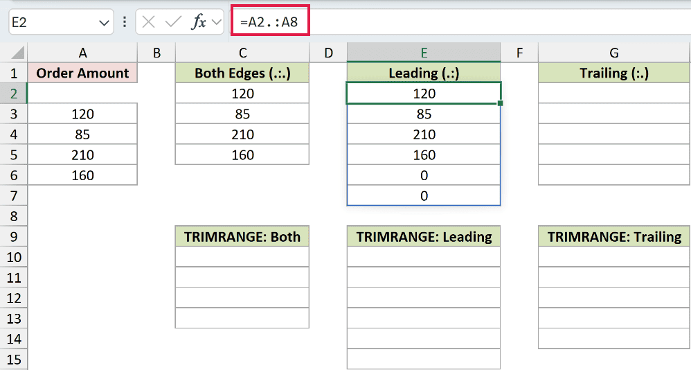
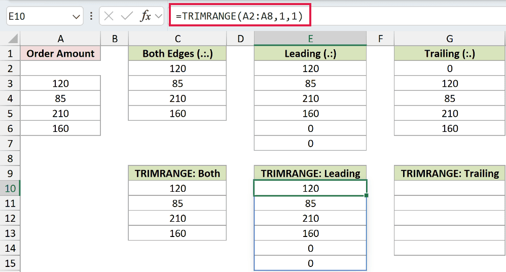
The .: operator trims leading blanks:
=A2.:A8
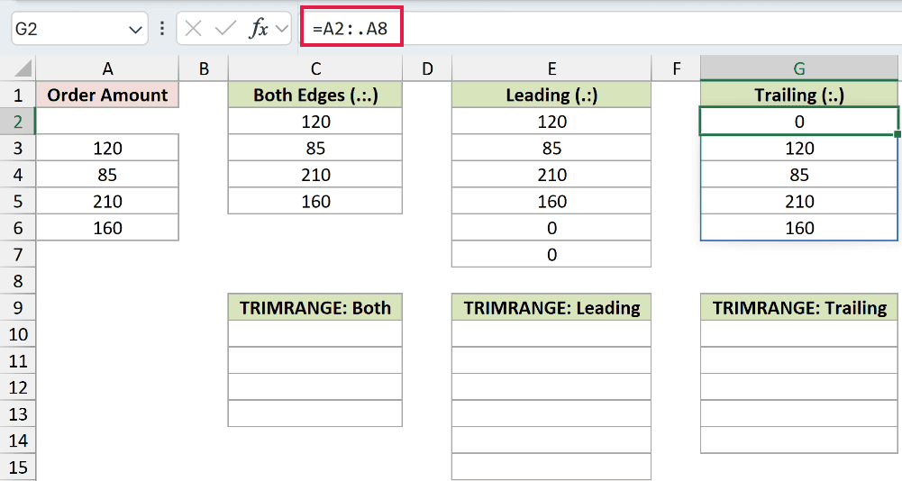
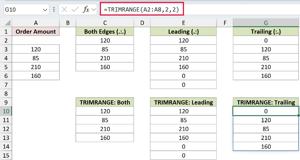
The :. operator trims trailing blanks:
=A2:.A8
Here is the equivalent TRIMRANGE formula for both edges:
=TRIMRANGE(A2:A8,3,3)
Here is the equivalent formula for leading blanks:
=TRIMRANGE(A2:A8,1,1)
And here is the equivalent formula for trailing blanks:
=TRIMRANGE(A2:A8,2,2)
- Both edges:
A2.:.A8andTRIMRANGE(A2:A8,3,3)return 120, 85, 210, and 160. - Leading edge:
A2.:A8andTRIMRANGE(A2:A8,1,1)return the four numbers followed by two blanks. - Trailing edge:
A2:.A8andTRIMRANGE(A2:A8,2,2)return one blank followed by the four numbers.
The retained blanks display as zeros in the spilled result. Each operator applies the same trim direction to rows and columns.
Use the full TRIMRANGE function when rows and columns need different settings, such as leading rows with both column edges in Example 2.
Tips & Common Mistakes
- Use Excel for Microsoft 365. Microsoft lists TRIMRANGE for Microsoft 365. It is not listed for Excel 2021 or Excel 2024.
- Keep the spill area clear. A blocked result produces a #SPILL! error.
- Expect a rectangle. TRIMRANGE stops at populated boundary cells and keeps everything inside that rectangular boundary.
- Do not expect interior cleanup. Blank rows or columns between populated records remain in the returned array.
- Delete blank records separately. Use these methods to remove blank rows when you want to change the source data.
- Choose row and column modes separately.
trim_rowsandtrim_colscan use different values in the same formula. - Read dot placement carefully.
.:.trims both edges,.:trims leading edges, and:.trims trailing edges. - Do not confuse TRIMRANGE with TRIM. TRIM removes extra spaces from text. TRIMRANGE removes blank outer rows and columns from a range or array.
- Use FILTER for criteria. TRIMRANGE does not test values or remove records based on a condition.
I use TRIMRANGE when an imported range has uncertain blank space around its edges. It returns a clean boundary while leaving the source untouched.
The examples also show where interior blanks remain and when trim references are a shorter option. I hope you found this article helpful.
