SORT Function in Excel

If you want to sort a list or table in Excel without touching the Sort button, the SORT function is what you’re looking for.

SORT is a dynamic array function, so it spills the sorted result into the cells below the formula and updates the moment your source data changes.

In this article, I’ll show you how to use SORT for ascending, descending, multi-column, and horizontal sorting, plus how it pairs with FILTER and UNIQUE.

One thing to flag right up front. SORT only works in Excel for Microsoft 365 and Excel 2021 (or later). If you’re on Excel 2019 or older, the function won’t be available and you’ll need to fall back to some alternate method.

SORT Syntax

Here is the syntax of the SORT function:

=SORT(array, [sort_index], [sort_order], [by_col])

• array – The range or array you want to sort.
• sort_index (optional) – The column or row number to sort by. Defaults to 1 (the first column or row).
• sort_order (optional) – 1 for ascending (default), -1 for descending.
• by_col (optional) – FALSE (default) sorts top to bottom by row. TRUE sorts left to right by column.

Only the first argument is required. The other three have sensible defaults, so a plain =SORT(A2:A10) gives you an ascending sort of that range.

When to Use SORT

Use this function when you need to:

• Return a sorted copy of a list or table without changing the original data.
• Build a dashboard or report where the sort needs to refresh automatically as data changes.
• Combine sorting with other formulas like FILTER or UNIQUE.
• Sort horizontally (across columns), which the Sort button can’t do without an extra step.

Let me show you a few practical examples of how to use the SORT function.

Example 1: Basic Ascending Sort

Let’s start with a simple example.

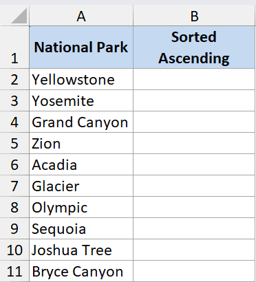
Below is a list of national park names in column A, and I want a sorted version of those names spilled into column C.

Here is the formula:

=SORT(A2:A11)

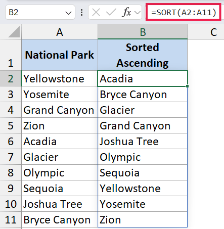
In the above formula, I’ve only passed the array argument. SORT defaults to sorting by the first column in ascending order, which is exactly what I want here. The result spills down from cell C2 into the cells below it.

If you add a new park to A2:A11, the sorted list in column C updates on its own. That’s the dynamic-array behavior at work.

Example 2: Sort in Descending Order

Here’s another practical scenario.

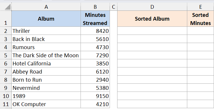
I have a list of albums and the total minutes streamed for each one, and I want to sort the entire table by streamed minutes from highest to lowest.

Here is the formula:

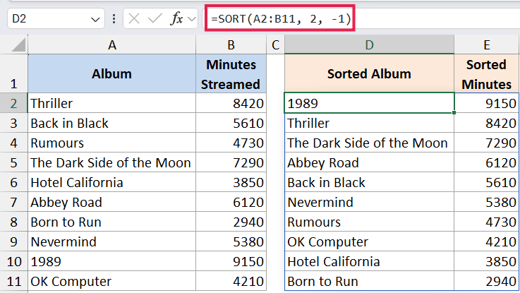
=SORT(A2:B11, 2, -1)

How this formula works:

• A2:B11 is the full table I want to sort, with the album titles in the first column and the streamed minutes in the second.
• 2 tells SORT to use the second column (minutes) as the sort key.
• -1 flips the order to descending, so the biggest number lands on top.

If I’d left the third argument out, SORT would have sorted ascending and put the smallest stream count first.

Example 3: Sort by a Specific Column

Now let’s look at something a bit more interesting.

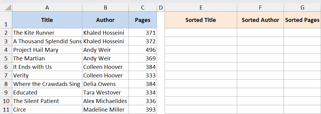
I have a book catalog with title in column A, author in column B, and page count in column C. I want to sort the whole table by author name, alphabetically.

Here is the formula:

=SORT(A2:C11, 2, 1)

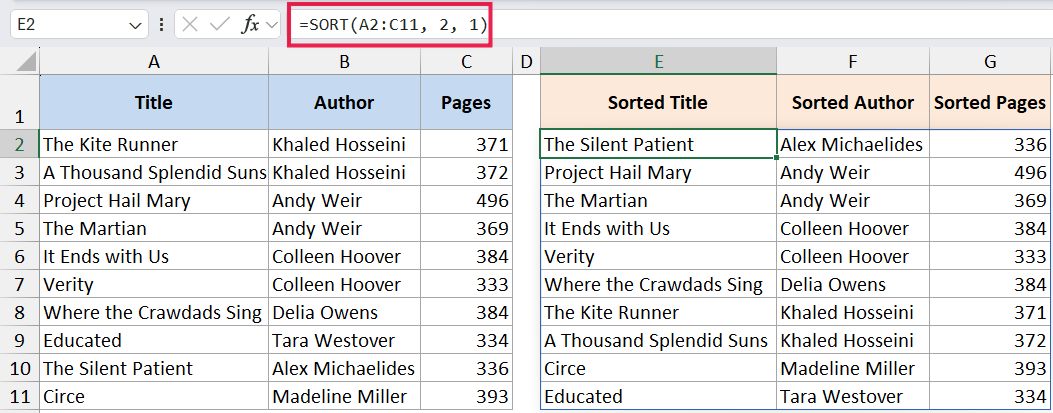
The 2 in the formula points SORT to the second column of the array, which is the author column. The 1 keeps the sort ascending (A to Z).

The titles and page counts follow their original rows, so each book stays attached to the right author after the sort.

Example 4: Multi-Column Sort

Let’s step it up with a more advanced use case.

Using the same book catalog, I want to first sort by author alphabetically, and then within each author, sort by page count from highest to lowest.

SORT only takes one value for sort_index, but you can pass an array constant to sort by more than one column.

Here is the formula:

=SORT(A2:C11, {2,3}, {1,-1})

How this formula works:

• {2,3} sorts first by column 2 (author), then by column 3 (page count).
• {1,-1} uses ascending order for the author and descending order for page count.
• The two arrays line up position by position, so the first sort key gets the first sort order, the second gets the second, and so on.

This is the dynamic-array equivalent of the multi-level Sort dialog box, but it stays live and updates whenever the source data changes.

Example 5: Sort Horizontally with by_col

Now here’s something the Sort button can’t do directly.

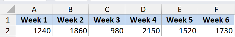
I have a row of weekly podcast download numbers in B2:G2, with week labels above them in B1:G1. I want to sort the weeks and their download values left to right, by downloads, from highest to lowest.

Here is the formula:

=SORT(B1:G2, 2, -1, TRUE)

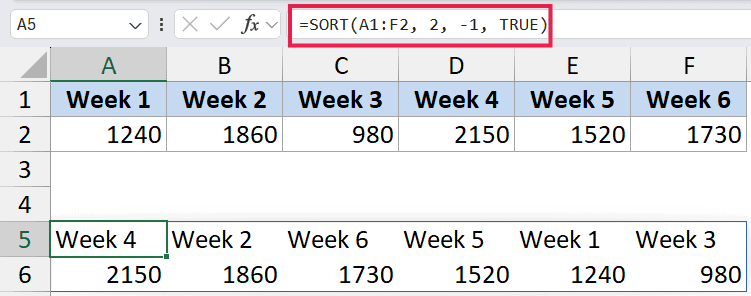
How this formula works:

• B1:G2 is the two-row range, week labels on top and downloads below.
• 2 picks the second row (downloads) as the sort key.
• -1 sorts from highest to lowest.
• TRUE flips the orientation so SORT works across columns instead of down rows.

Without that fourth argument set to TRUE, SORT would try to sort top to bottom and you’d get back the same range you started with.

Example 6: SORT with FILTER and UNIQUE

This is one of my favorite combinations.

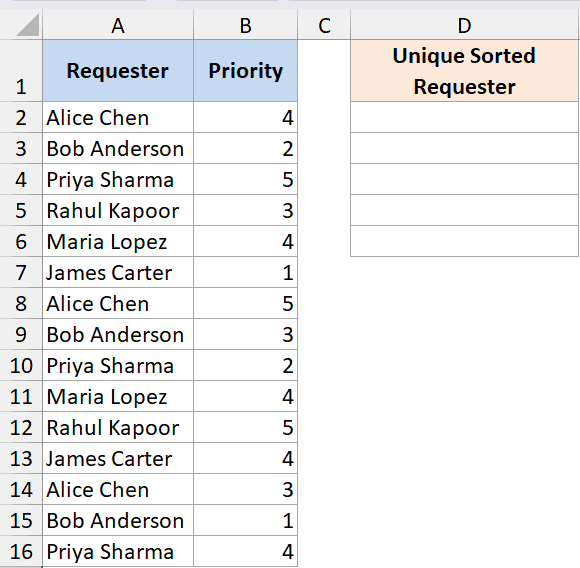
I have a support-ticket log where the same requester can file multiple tickets. I want a clean, sorted, deduplicated list of requesters, but only the ones who logged a ticket with priority above 3.

Here is the formula:

=SORT(UNIQUE(FILTER(A2:A50, B2:B50>3)))

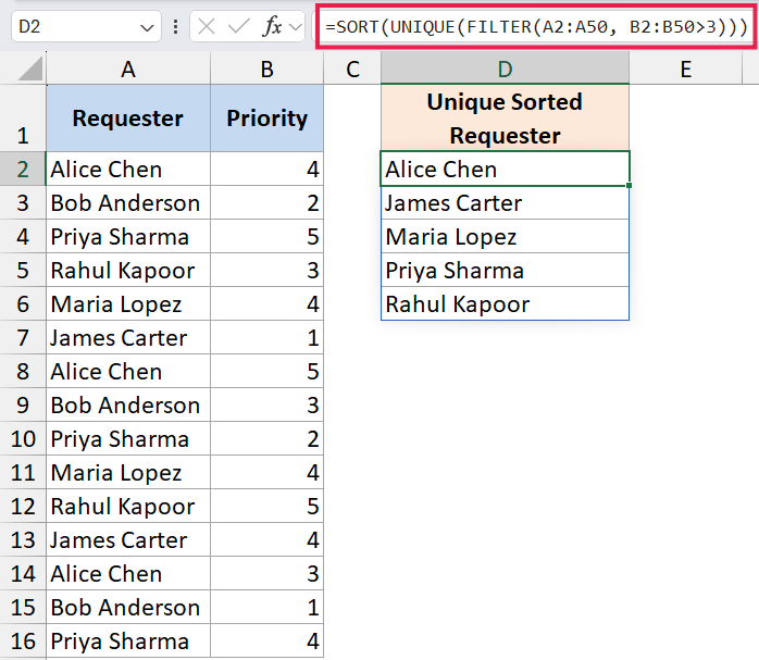
How this formula works:

• FILTER(A2:A50, B2:B50>3) keeps only the requesters whose ticket priority is greater than 3.
• UNIQUE(…) strips out duplicate names from that filtered list. If you’d like a refresher, here’s how to get unique values from a column.
• SORT(…) wraps the whole thing and returns the final list in alphabetical order.

The three functions chain together in one formula and give you a live, sorted, deduplicated, filtered list. No helper columns, no manual cleanup.

SORT vs SORTBY: Which One to Use

SORT and SORTBY look similar, but they solve slightly different problems.

• SORT sorts an array using a column or row inside that array. You pass it a sort_index number.
• SORTBY sorts an array using one or more separate ranges as the sort key. The sort key doesn’t need to be part of the array you’re returning.

A quick example. If you want to sort a list of names by a separate column of birthdays, but only return the names, SORTBY is cleaner:

=SORTBY(A2:A11, C2:C11, 1)

If the sort key is already inside the table you’re returning, SORT is the simpler choice.

Use SORTBY when the sort key sits in a column you don’t want in the output, or when you’re sorting by a calculated array. Use SORT for everything else.

SORT Function vs the Sort Button

The Sort button on the Data tab and the SORT function both sort data, but they behave very differently.

• Sort button rearranges the original data in place. It’s a one-time action. If your source data changes, you have to sort again.
• SORT function returns a sorted copy in a different range. The original data stays untouched, and the result updates automatically when the source changes.

I reach for the Sort button when I’m doing a quick one-off sort and don’t care about keeping the original order. I reach for the SORT function when I’m building a dashboard, summary, or any report where the data feeds into something else and needs to stay current.

Tips & Common Mistakes

• #SPILL! error: SORT spills its result into the cells below or to the right of the formula. If any of those cells already have data, you’ll get a #SPILL! error. Clear the spill range and the formula will work.
• Reference the spilled result with #: If your SORT lives in cell C2, refer to its full output as C2# in any downstream formula. The reference resizes automatically when the sorted output grows or shrinks.
• @ implicit intersection collapses the spill: Older Excel versions sometimes auto-insert an @ symbol when they save a workbook (e.g. =@SORT(...)). That collapses the result to a single cell. Remove the @ and the spill comes back.
• Not available in older Excel: SORT only exists in Microsoft 365 and Excel 2021 or later. If you open a file containing SORT in Excel 2019 or earlier, you’ll see _xlfn._xlws.SORT and the cell will show a #NAME? error.
• sort_order must be 1 or -1: Any other number, like 2 or 0, returns a #VALUE! error. Stick to 1 for ascending and -1 for descending.
• sortindex out of range: If you pass a sortindex larger than the number of columns (or rows, when by_col is TRUE) in the array, you’ll get a #VALUE! error.
• SORT inside an Excel Table: SORT and other dynamic-array functions don’t play nicely inside a formatted Excel Table. Put the formula in a regular range, or convert the table back to a range first.
• Original data is untouched: SORT returns a new sorted array. It doesn’t reorder the source range. If you actually want to overwrite the original order, use the Sort button or copy the SORT result and paste it back as values.

The SORT function is one of the more useful additions in newer versions of Excel. Once you start using it for ascending, descending, and multi-column sorts, plus combinations with FILTER and UNIQUE, the Sort button starts to feel pretty limited for anything that needs to stay live.

And when the sort key sits outside the range you want to return, SORTBY picks up where SORT leaves off.

List of All Excel Functions

Other Excel articles you may also like:

• Sort by Date in Excel (Single Column & Multiple Columns)
• How to Sort by Length in Excel? (Formula)
• How to Flip Data in Excel (Columns, Rows, Tables)?
• How to Unsort in Excel (Revert Back to Original Data)