DAVERAGE Function in Excel

The DAVERAGE function in Excel returns the average of a database field for records that match conditions in a separate criteria range.

Keeping the conditions in worksheet cells makes them easier to inspect or change without editing the formula.

Conditions on the same criteria row work together. Conditions on different rows create alternatives, so the layout determines which records contribute to the average.

In this article, I’ll show you how to average records using AND or OR criteria, apply a numeric band, and use formula-based criteria.

DAVERAGE Function Syntax in Excel

DAVERAGE averages a selected field for records that meet the criteria you specify.

=DAVERAGE(database,field,criteria)

• database is the complete range, including its header row.
• field is the field name in double quotes or its one-based position in the database.
• criteria is a headered range containing at least one condition cell below the header.

When to Use DAVERAGE Function

• Average records that meet editable worksheet criteria.
• Keep criteria separate from a larger database table.
• Combine several conditions without nesting IF functions.
• Reuse a criteria block with other database functions.

Example 1: Text Criteria and Exact Match

Let’s start with a visible text criterion.

Below is an audit database with a Store Format criteria block beside it.

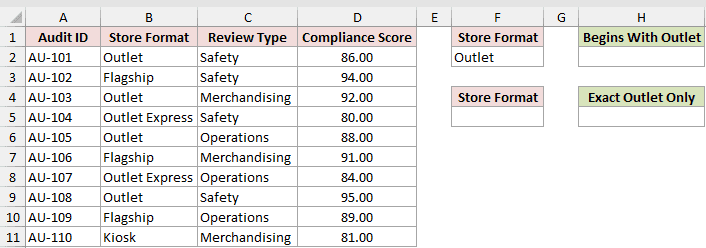
I want the average compliance score for store formats beginning with Outlet.

Here is the formula:

=DAVERAGE(A1:D11,"Compliance Score",F1:F2)

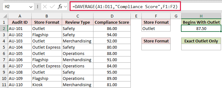
The text criterion in F2 is Outlet. Without an equal sign, it matches Outlet and Outlet Express, so the average is 87.50.

Now I want an exact match for Outlet only.

Here is the criterion formula:

="=Outlet"

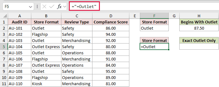
Excel displays =Outlet in the criterion cell. The formula is needed because typing it directly would make Excel treat it as a calculation.

Here is the exact-match DAVERAGE formula:

=DAVERAGE(A1:D11,"Compliance Score",F4:F5)

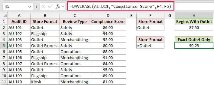
The exact-match result is 90.25. It includes only the two rows whose Store Format is exactly Outlet.

Example 2: AND Criteria in Different Fields

Criteria on the same row work together as AND conditions.

Below is a service-operations database with Team and Service Level criteria.

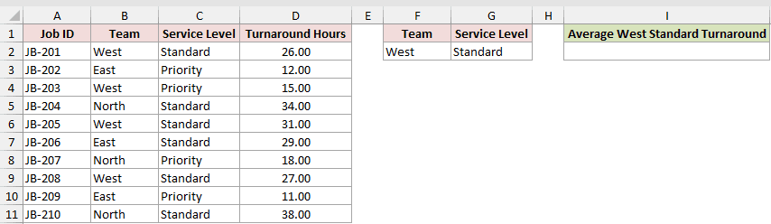
I want the average turnaround for West team jobs that also have the Standard service level.

Here is the formula:

=DAVERAGE(A1:D11,4,F1:G2)

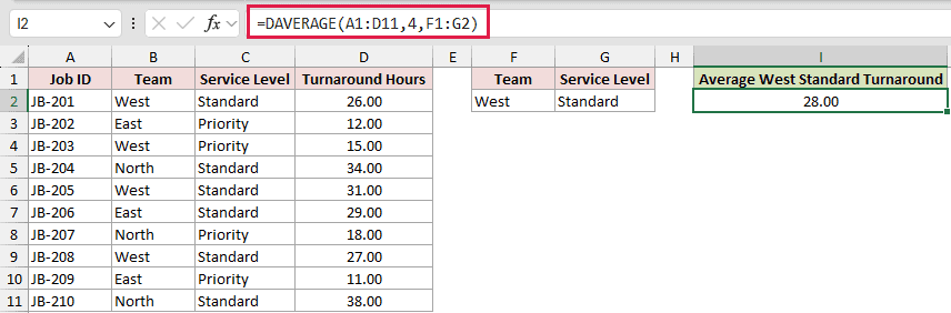
The field argument is 4, which refers to Turnaround Hours, the fourth database column.

Because West and Standard are on the same criteria row, a record must meet both conditions. The result is 28.00 hours.

Example 3: OR Criteria in One Field

Putting criteria on separate rows changes the logic.

Below is a grant-reporting database with two program names under the same heading.

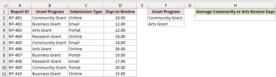
I want the average review time for Community Grant or Arts Grant submissions.

Here is the formula:

=DAVERAGE(A1:D11,"Days to Review",F1:F3)

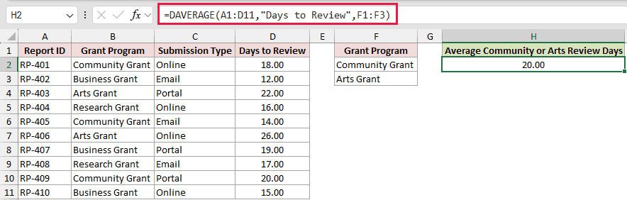
The entries in F2 and F3 sit in separate rows. DAVERAGE therefore includes records matching either program.

The average review time is 20.00 days.

Example 4: Average Values in a Numeric Band

You can repeat a header to apply two tests to one field.

Below is a parcel database with a criteria block for handling costs between $45 and $90.

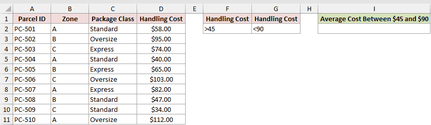
I want the average handling cost for parcels above $45 and below $90.

Here is the formula:

=DAVERAGE(A1:D11,"Handling Cost",F1:G2)

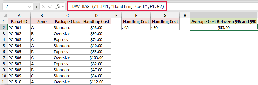
The repeated Handling Cost headers let the two criteria apply to the same record. F2 contains >45, and G2 contains <90.

The qualifying costs are $58, $74, $65, $82, and $47. Their average is $65.20.

Example 5: Use a Formula Criterion

A formula criterion can test every record against a calculated benchmark.

Below is a support-case database with a separate formula criterion cell.

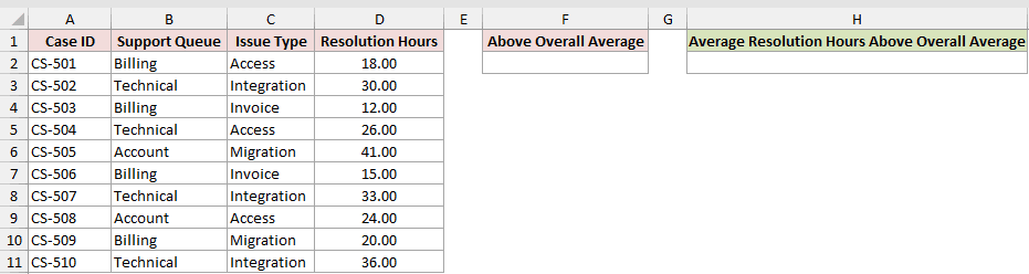
I want to include only cases whose resolution hours are above the overall average.

Here is the criterion formula:

=D2>AVERAGE($D$2:$D$11)

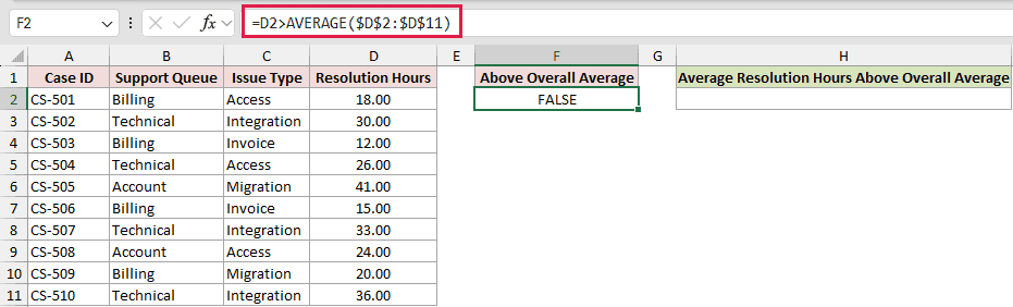
D2 is a relative reference to the first data record. The full comparison range stays absolute, so Excel evaluates each row against the same overall average.

Here is the DAVERAGE formula:

=DAVERAGE(A1:D11,"Resolution Hours",F1:F2)

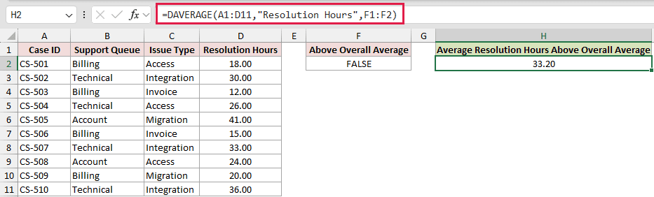
The criterion heading in F1 does not match a database header. That tells DAVERAGE it is a formula criterion.

The selected cases average 33.20 resolution hours.

Example 6: Use a Spilled Criteria Range

This example uses a dynamic array to build the criteria block, while DAVERAGE still returns one average.

Below is a training-cohort database with an editable minimum-rating value in J2.

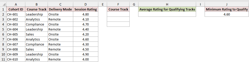
I want to create a criteria list of course tracks with at least one session rated 4.6 or higher.

Here is the formula:

=VSTACK("Course Track",UNIQUE(FILTER(B2:B11,D2:D11>=J2)))

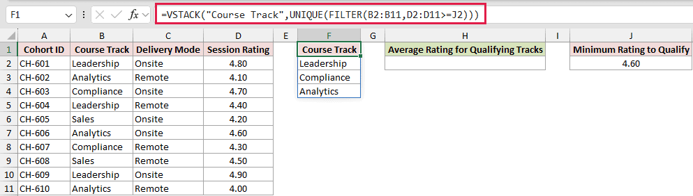
FILTER keeps tracks with a qualifying session. UNIQUE removes duplicates, and VSTACK adds the required Course Track header above the spilled criteria.

Now I want the average rating for every record in those qualifying tracks.

Here is the formula:

=DAVERAGE(A1:D11,"Session Rating",F1#)

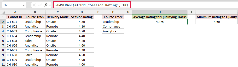
F1# refers to the complete spilled criteria range. The result is 4.475.

For a simple one-off conditional average, AVERAGEIFS is often more direct. DAVERAGE is useful when you want editable criteria blocks.

Tips & Common Mistakes

• Include the header row in the database range.
• Keep the criteria range separate from the database. Do not let the two ranges overlap.
• Criteria on the same row are AND conditions. Criteria on different rows are OR conditions.
• A plain text criterion can match values that begin with that text. Use a displayed =text criterion for an exact text match.
• Wildcards work in text criteria: * matches any number of characters, ? matches one, and ~ escapes a wildcard.

DAVERAGE is useful when your criteria need to stay visible and easy to edit. I hope you found this article helpful.

List of All Excel Functions

Other Excel articles you may also like:

• DCOUNTA function
• DVAR Function in Excel