
Excel’s AVERAGEIFS function returns the arithmetic mean of cells that meet all the conditions you specify.
It helps compare results for a particular category, date range, or combination of criteria. Only matching numeric values in the average range contribute to the result.
In this article, I’ll show you how to combine criteria, average values between dates, and handle zeros or groups with no matching numbers.
AVERAGEIFS Function Syntax in Excel
Here is the syntax for the AVERAGEIFS function:
=AVERAGEIFS(average_range, criteria_range1, criteria1, [criteria_range2, criteria2], ...)
- average_range is the range containing the numbers you want to average.
- criteria_range1 is the first range Excel checks.
- criteria1 is the condition applied to criteria_range1.
- criteria_range2, criteria2 are optional additional range-and-condition pairs. You can use up to 127 pairs.
AVERAGEIFS applies AND logic. A row must meet every condition before its value from average_range enters the calculation.
Every criteria range must have the same dimensions as average_range. Mismatched ranges return a #VALUE! error.
When to Use AVERAGEIFS Function
- You need an average based on two or more text, number, or date conditions.
- You want to combine exact matches with operators such as greater than, less than, or not equal to.
- You need partial text matching with wildcards.
- You want criteria stored in worksheet cells so users can change them easily.
- You need one conditional average for each item in a spilled list.
Example 1: Average Wages With Two Text Criteria
Let’s start with two straightforward text conditions.
Below is the dataset of employees, stores, roles, and hourly wages in columns A through D.
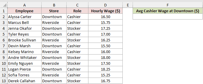
We want the average hourly wage for cashiers working at the Downtown store.
Here is the formula:
=AVERAGEIFS(D2:D13,B2:B13,"Downtown",C2:C13,"Cashier")
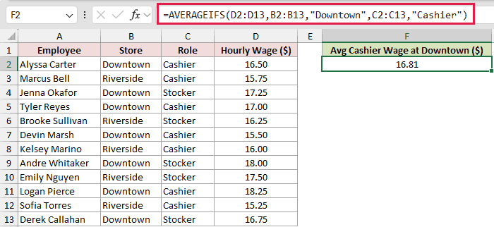
The formula returns $16.81. Four rows match both conditions, with wages of $16.50, $17.00, $15.50, and $18.25.
D2:D13 contains the wages to average. Excel checks B2:B13 for Downtown and C2:C13 for Cashier. Only rows that pass both tests remain.
Example 2: AVERAGEIFS With Greater Than Criteria
Here’s a practical example using two numeric comparisons.
Below is the dataset of servers, party sizes, bill totals, and tip percentages in columns A through D.
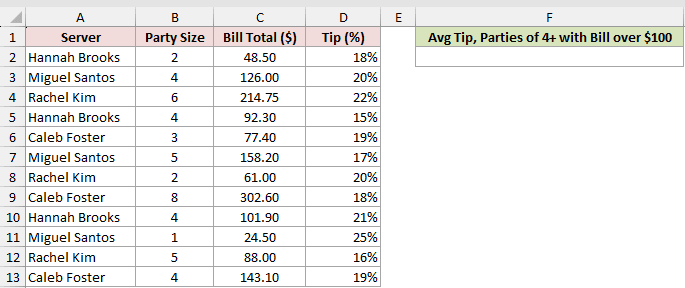
We want the average tip percentage for parties of four or more whose bill exceeded $100.
Here is the formula:
=AVERAGEIFS(D2:D13,B2:B13,">=4",C2:C13,">100")
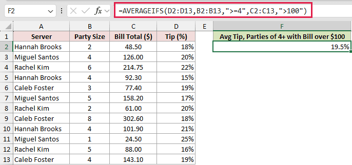
The result is 19.5%. Six bills meet both thresholds, and their tip percentages are 20%, 22%, 17%, 18%, 21%, and 19%.
Comparison operators belong inside quotation marks. The first condition includes parties of four, while the second condition excludes bills equal to exactly $100.
Pro Tip: Use “>=4” when four should count. Use “>4” when the value must be strictly greater than four.
Example 3: Average Between Two Dates
Now let’s combine a date window with a text condition.
Below is the dataset of appointment dates, clinics, and wait times, followed by criteria cells in columns E through G.
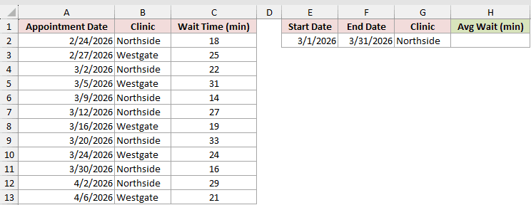
We want the average March 2026 wait time at the Northside clinic.
Here is the formula:
=AVERAGEIFS(C2:C13,A2:A13,">="&E2,A2:A13,"<="&F2,B2:B13,G2)
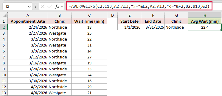
The formula returns 22.4 minutes. It averages the five Northside appointments dated from March 1 through March 31, including both boundary dates.
The operators stay inside quotation marks and join the date cells with ampersands. G2 supplies the clinic name, so changing the criteria cells updates the result.
Example 4: AVERAGEIFS With Wildcard Criteria
Here’s how to average rows that begin with matching text.
Below is the dataset of course titles, formats, and average ratings in columns A through C.
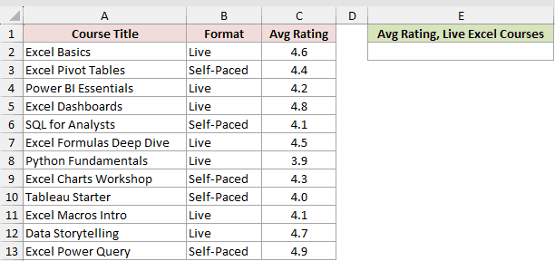
We want the average rating for Live courses whose titles start with Excel.
Here is the formula:
=AVERAGEIFS(C2:C13,A2:A13,"Excel*",B2:B13,"Live")
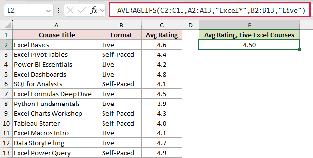
The result is 4.50. Excel Basics, Excel Dashboards, Excel Formulas Deep Dive, and Excel Macros Intro meet both conditions.
The asterisk matches any text after Excel. It does not affect the separate Live condition, which must also match on the same row.
Pro Tip: An asterisk matches any number of characters. A question mark matches exactly one character, and a tilde lets you match a literal wildcard.
Example 5: Fix the #DIV/0! Error With IFERROR
Let’s see what happens when no row meets every condition.
Below is the dataset of gym classes, instructors, and attendance, with the requested instructor and class in E2 and F2.
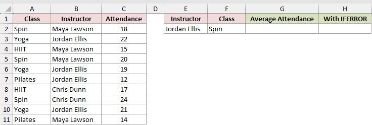
We want Jordan Ellis’s average attendance for Spin classes, although the dataset contains no such row.
Here is the formula:
=AVERAGEIFS(C2:C11,B2:B11,E2,A2:A11,F2)
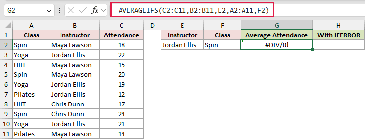
The formula returns #DIV/0! because Jordan Ellis never teaches a Spin class in this dataset.
To show a helpful message instead, wrap the same formula in IFERROR:
=IFERROR(AVERAGEIFS(C2:C11,B2:B11,E2,A2:A11,F2),"No classes found")
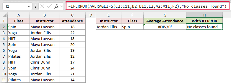
The second formula returns “No classes found”. IFERROR is the cleaner option when an empty match is expected and readers need a clear message.
Use this carefully. IFERROR catches every error, so it can also hide a broken range or another formula problem you should fix.
Example 6: Blank Cells vs. Zeros in AVERAGEIFS
Here’s a delivery example with a day off and a breakdown day.
Below is the dataset of delivery drivers, routes, and packages delivered, including a blank day off and a zero caused by a van breakdown.
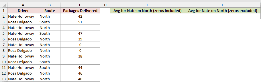
We want Nate Holloway’s North route average, first with zeros included and then with zeros excluded.
Here is the formula:
=AVERAGEIFS(C2:C13,A2:A13,"Nate Holloway",B2:B13,"North")
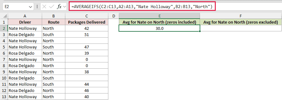
This returns 30.0 packages. AVERAGEIFS skips the blank average-range cell but includes the numeric zero. That zero pulls the average down.
Here is the formula that excludes zeros:
=AVERAGEIFS(C2:C13,A2:A13,"Nate Holloway",B2:B13,"North",C2:C13,"<>0")
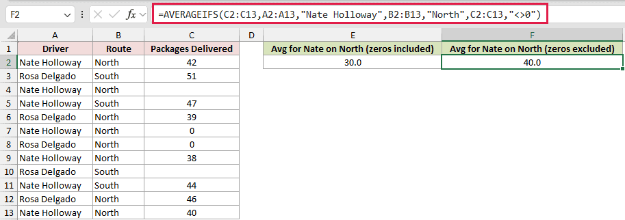
The added condition keeps only nonzero deliveries. The result becomes 40.0, based on 42, 38, and 40 packages.
Here, the breakdown day is a real zero, while the blank marks a day off. Excluding zero would leave out an actual delivery result.
Example 7: Spilled Group Averages and OR Logic
Finally, let’s combine AVERAGEIFS with dynamic array formulas.
Below is the dataset of room types, seasons, and nightly rates, with output areas for grouped averages and a combined OR calculation.
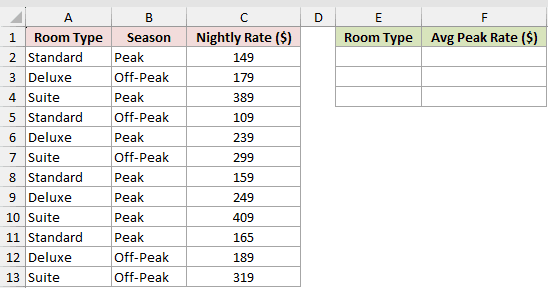
We want one Peak average per room type, followed by one Peak average covering Suite or Deluxe rooms.
Here is the formula:
=UNIQUE(A2:A13)
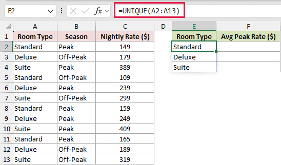
UNIQUE spills Standard, Deluxe, and Suite into E2:E4.
Next, use that spilled list as the AVERAGEIFS criteria:
=AVERAGEIFS(C2:C13,A2:A13,E2:E4,B2:B13,"Peak")
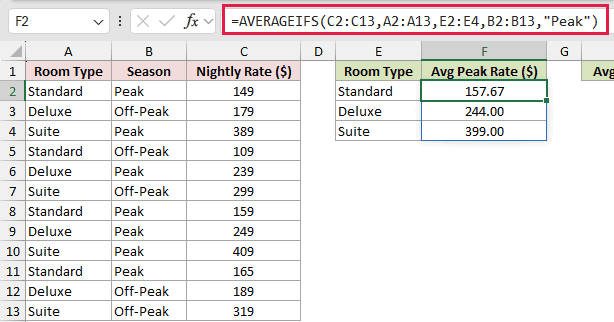
The formula spills three results: $157.67 for Standard, $244.00 for Deluxe, and $399.00 for Suite.
AVERAGEIFS uses AND logic, so FILTER is more direct when either Suite or Deluxe can match:
=AVERAGE(FILTER(C2:C13,((A2:A13="Suite")+(A2:A13="Deluxe"))*(B2:B13="Peak")))
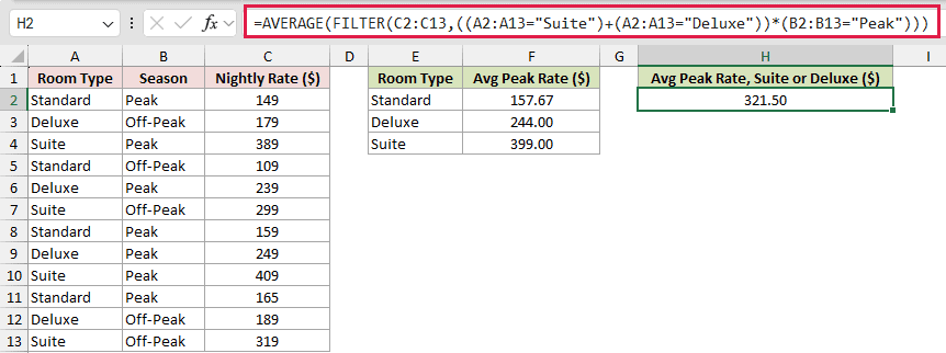
The result is $321.50. The plus sign joins Suite and Deluxe with OR logic, while multiplication requires the Peak condition too.
In Excel 365, GROUPBY can return one average per room type more directly. The spilled AVERAGEIFS approach still works and remains useful when you need several criteria.
Tips & Common Mistakes
- Keep every criteria range the same size and shape as average_range. Unlike AVERAGEIF, AVERAGEIFS requires matching dimensions.
- Put comparison operators inside quotation marks. When a value comes from a cell, join the operator and cell reference with an ampersand.
- Use AVERAGEIF when you only have one condition. AVERAGEIFS still works, but its extra range-and-condition structure is unnecessary.
- Remember that AVERAGEIFS uses AND logic. Use AVERAGE with FILTER when you need OR logic in Excel 365.
- Text and blank cells in average_range are ignored. Numeric zeros are averaged unless you exclude them with another condition.
- A #DIV/0! error usually means no rows matched or the matching average cells contained no numbers.
- Text criteria are not case-sensitive, including wildcard matches. Use a tilde before an asterisk or question mark when you need the literal character.
I use AVERAGEIFS whenever an average should include only rows that meet several conditions.
The examples above cover the cases I reach for most often, including empty matches and grouped averages.
I hope you found this article helpful.
Related Excel Functions / Articles:
Other Excel articles you may also like:
