
Excel’s SKEW function returns the skewness of a sample, which describes how asymmetrically its values spread around the mean.
A positive result points to a longer tail toward larger values. A negative result points to a longer tail toward smaller values. Values near zero suggest greater symmetry.
In this article, I’ll show you how to interpret positive and negative skewness, compare samples, and check how an unusual value affects the SKEW result.
SKEW Function Syntax in Excel
SKEW accepts separate numbers, arrays, or cell references containing sample data.
=SKEW(number1, [number2], ...)
number1is the first required number, array, or reference.number2, through additional arguments, are optional numbers, arrays, or references. Excel accepts up to 255 numeric arguments.
When to Use SKEW Function
- Measure whether a sample has a longer right or left tail.
- Compare the asymmetry of two samples.
- Calculate skewness for a filtered subset.
- Check whether sample and population formulas are being used correctly.
- See whether an unusual observation is strongly affecting a distribution.
Example 1: Measure Positive Skewness
A single large value can create a visible right tail.
Below is the dataset with donation IDs, gift amounts, and the sample skewness result.
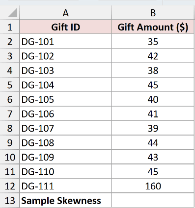
We want to measure the asymmetry of the gift amounts in B2:B12.
Here is the formula:
=SKEW(B2:B12)
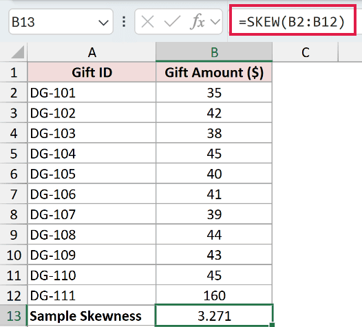
The formula returns 3.271. Most gifts sit between $35 and $45, while one $160 gift extends the tail toward larger values.
The positive sign describes the tail’s direction. It does not mean that the data is good or bad.
Pro Tip: Interpret SKEW with the source values in view. The number describes asymmetry, but the dataset shows what is creating it.
Example 2: Compare Positive and Negative Skew
Two samples can have tails in opposite directions.
Below is the dataset with two release tracks and their resolution hours.
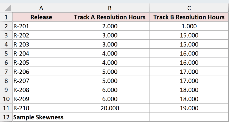
We want to calculate and compare the sample skewness of both tracks.
Here is the formula for Track A:
=SKEW(B2:B11)
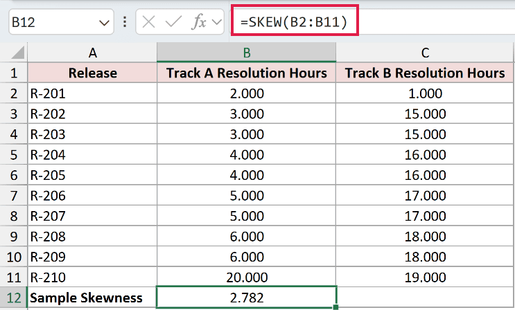
Track A returns 2.782. Its 20-hour value stretches the distribution toward larger values.
Here is the formula for Track B:
=SKEW(C2:C11)
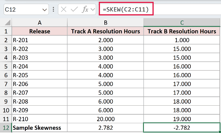
Track B returns -2.782. Its 1-hour value stretches the distribution toward smaller values.
The equal magnitudes reflect the mirrored data, while the signs identify the different tail directions.
Example 3: Calculate Skewness for a Group
SKEW can reduce a filtered array to one result.
Below is the dataset with priority and standard contract reviews, their hours, and a priority-only skewness result.
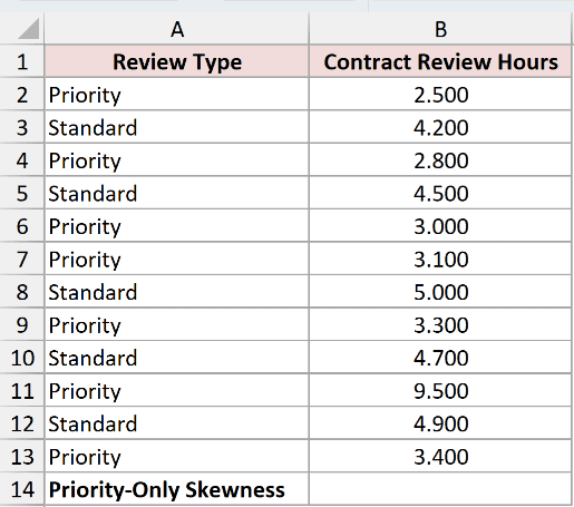
We want to measure skewness using only rows marked Priority.
Here is the formula:
=SKEW(FILTER(B2:B13,A2:A13="Priority"))
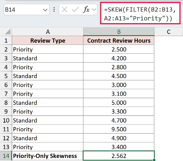
The FILTER function returns the eight priority review times. SKEW reduces that array to one value and returns 2.562.
The 9.5-hour priority review creates a longer tail toward larger values. Standard-review rows do not enter this calculation.
Pro Tip: FILTER is available in Excel 2021, Excel 2024, and Microsoft 365. Older versions need a separate range containing the selected group’s values.
Example 4: Compare SKEW and SKEW.P
The scope of the data determines which function belongs in the analysis.
Below is the dataset with ten audit readings and both sample and population skewness results.
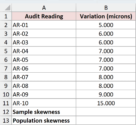
We want to compare the sample formula with the population formula for the same values.
Here is the sample formula:
=SKEW(B2:B11)
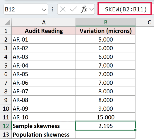
SKEW treats the ten readings as a sample from a larger group and returns 2.195.
Here is the population formula:
=SKEW.P(B2:B11)
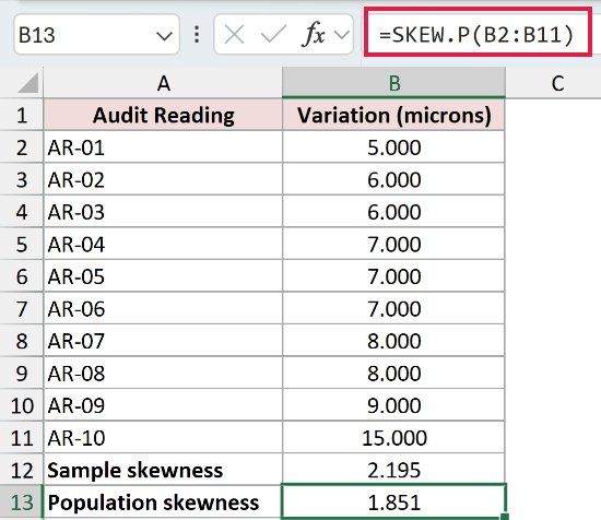
SKEW.P treats the ten readings as the complete population and returns 1.851.
Choose between these formulas from how the data was collected, not from which result looks more useful.
Pro Tip: Use SKEW for a sample and SKEW.P for a complete population. The function choice comes from the data scope.
Example 5: Check an Outlier’s Effect
Comparing the result with and without one unusual case can explain a large skewness value.
Below is the dataset with all repair jobs, routine jobs, and a separate refurbishment project.
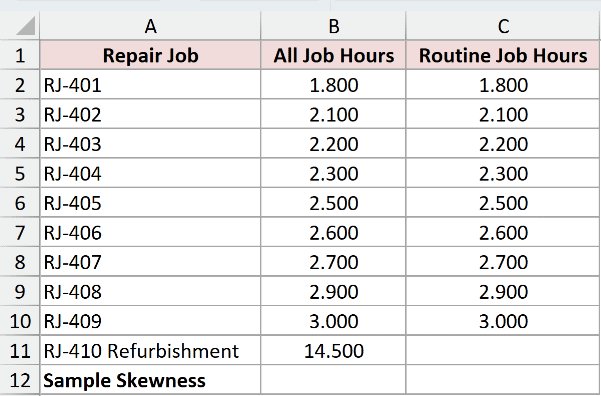
We want to compare skewness for all jobs with skewness for routine jobs only.
Here is the formula using every job:
=SKEW(B2:B11)
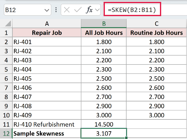
Including the 14.5-hour refurbishment job produces a skewness of 3.107.
Here is the formula using the routine jobs:
=SKEW(C2:C10)
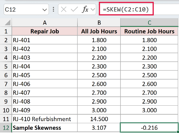
The routine jobs return -0.216, which is much closer to zero. The comparison shows how strongly the refurbishment job affects the full sample.
Check whether an unusual value is an outlier before removing it. A valid rare event may be important even when it changes the distribution sharply.
Tips & Common Mistakes
- SKEW returns one value for an array or range. It is a reducer and does not spill one result per source row.
- Positive and negative signs describe tail direction. They are not quality scores.
- Use SKEW for sample data and SKEW.P for a complete population.
- Excel ignores text, logical values, and blanks inside a referenced range, but it includes cells containing zero.
- SKEW needs at least three numeric values with some variation. Fewer than three values or zero sample standard deviation returns
#DIV/0!. - A large skewness result can point to an outlier, but it does not prove that the value is an error.
I covered tail direction, comparison samples, filtered groups, sample versus population formulas, and the effect of an unusual observation.
I hope you found this article helpful.
Related Excel Functions / Articles:
