The STDEV function measures how spread out a set of numbers is, giving you the sample standard deviation. A small result means the values sit close to the average, and a big result means they swing around a lot. This article walks through real examples so you can see exactly how it behaves.
STDEV returns a single value, but it works fine inside dynamic array formulas, for example =STDEV(FILTER(...)) to measure just one group. One key point before you start: STDEV is the legacy function, while STDEV.S (sample) and STDEV.P (population) are the modern versions.
STDEV Function Syntax in Excel
Here is how the STDEV function is written.
=STDEV(number1, [number2], ...)
- number1 (required): the first value or range you want to measure.
- number2, … (optional): more values or ranges to include.
It accepts a range like B2:B11 and uses the sample method, which divides by n-1. It also ignores text and empty cells in the range.
When to Use STDEV Function
- Measure the variability of test scores across a class.
- Track sales volatility from one month to the next.
- See the spread in a set of physical measurements.
- Check consistency in quality control, where steady output matters.
- Compare the consistency of two datasets side by side.
Example 1: Basic Sample Standard Deviation
Let’s start with the simplest case, a single column of scores.
Below is the dataset with student names in column A and their test scores in column B.
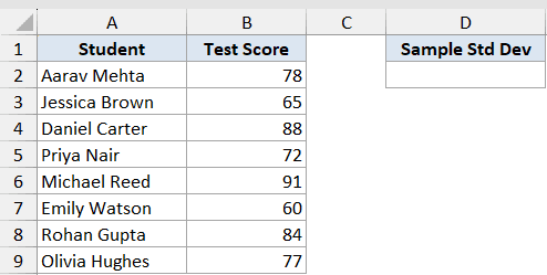
We want to measure how much the test scores vary around the average.
Here is the formula:
=STDEV(B2:B9)
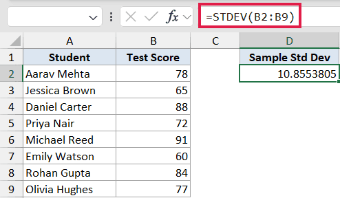
The result is about 10.86. A higher number means more spread, so here the scores swing roughly 11 points around the mean. If everyone scored close to the same mark, this number would be much smaller.
Example 2: Sample vs Population
Sometimes you need to decide whether your data is a sample or the whole population. This example shows both side by side.
Below is the dataset with machine names in column A and their daily output in column B. To the right is a small block with “Measure” and “Result” rows.
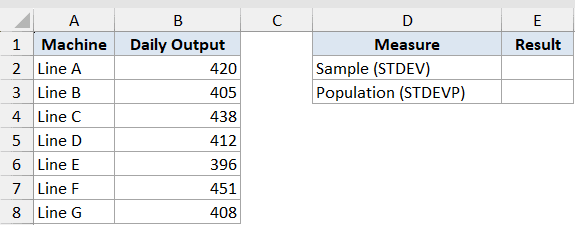
We want to compare the sample and population standard deviation on the same data.
Here is the formula:
=STDEV(B2:B8)
=STDEVP(B2:B8)
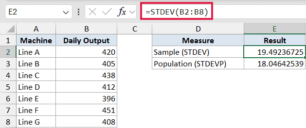
STDEV returns about 19.49 and STDEVP returns about 18.05. STDEV divides by n-1 (sample), which makes it slightly larger. STDEVP divides by n (population). The modern equivalents are STDEV.S and STDEV.P. Choose sample when the data is a subset, and population when it is everything you have.
Pro Tip: Use STDEV / STDEV.S when your data is a sample of a bigger group, and use STDEVP / STDEV.P when you have the whole population.
Example 3: STDEV Ignores Text and Blanks
Real data is rarely clean, so let’s see what happens with a blank cell and a text entry in the range.
Below is the dataset with sales rep names in column A and their monthly sales in column B. One cell is blank and one holds the text “N/A”.
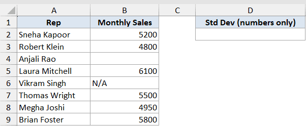
We want to see what STDEV does when the range has a blank cell and a text entry.
Here is the formula:
=STDEV(B2:B9)
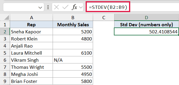
The result is about 502.41. The blank cell and the “N/A” text are skipped automatically, so the calculation runs on the 6 numeric values only. No error is shown, which is handy but easy to miss.
Pro Tip: Numbers stored as text are skipped too, so a column that looks numeric can quietly compute on fewer points than you think.
Example 4: Compare Consistency of Two Datasets
Standard deviation shines when you put two sets next to each other. Here we compare two suppliers.
Below is the dataset with the week in column A, Supplier X volumes in column B, and Supplier Y volumes in column C. To the right is a “Measure” and “Std Dev” block.
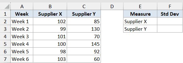
We want to find out which supplier delivers more consistent volumes.
Here is the formula:
=STDEV(B2:B7)
=STDEV(C2:C7)
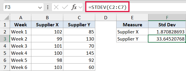
Supplier X comes in around 1.87 and Supplier Y around 33.65. The lower standard deviation means Supplier X delivers steadier output. Supplier Y swings a lot week to week, even if the two averages look similar.
Example 5: Standard Deviation of a Filtered Subset
You can feed STDEV a dynamic array so it measures just one slice of your data. This example pulls one region.
Below is the dataset with salesperson names in column A, revenue in column B, and region in column C.
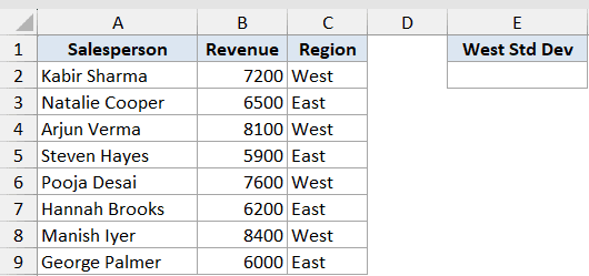
We want to measure the spread of revenue for the West region only.
Here is the formula:
=STDEV(FILTER(B2:B9,C2:C9="West"))
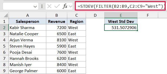
The result is about 531.51. The FILTER function pulls just the West revenue values into a dynamic array, and STDEV reduces them to one number. This is the dynamic-array composition, where STDEV acts as a reducer that works inside other formulas. This needs Excel 365.
Tips & Common Mistakes
- Pick the right version: STDEV / STDEV.S for a sample (a subset you’re estimating from), STDEVP / STDEV.P when the data is the entire population.
- STDEV ignores text, logical values, and empty cells in a range, so check your data really has the count of numbers you expect. STDEVA includes text and logicals if you need that.
- STDEV needs at least two numeric values. A single value returns a #DIV/0! error.
- Numbers stored as text are skipped, which quietly shrinks your sample. Convert them to real numbers first.
- STDEV and STDEVP are the legacy names kept for compatibility. STDEV.S and STDEV.P are clearer and recommended for new workbooks.
That covers the main ways to put STDEV to work, from a plain column of scores to a filtered subset. The function itself is simple, and the real skill is picking sample versus population and keeping your data clean. Once that clicks, you can read the spread in any dataset at a glance.
Related Excel Functions / Articles: