
Excel’s CHISQ.TEST function returns the p-value from a chi-square comparison between observed and expected frequencies. It does not return the chi-square statistic itself.
Excel infers the degrees of freedom from the shape of the ranges, so there is no separate degrees-of-freedom argument.
In this article, I’ll show you how to test an equal split, compare a benchmark mix, analyze contingency tables, and work from raw survey responses.
CHISQ.TEST Function Syntax in Excel
The CHISQ.TEST function uses the following syntax:
=CHISQ.TEST(actual_range, expected_range)
actual_rangeis the range containing the observed frequencies.expected_rangeis the equally sized range containing the expected frequencies.
When to Use CHISQ.TEST Function
- Check whether observed category counts follow an expected distribution.
- Compare this year’s category mix with a historical or planned benchmark.
- Test whether two categorical variables are associated in a contingency table.
- Return a p-value after calculating expected counts from row and column totals.
Example 1: Chi-Square Goodness-of-Fit Test
Let’s start with an equal-distribution test.
Below is the dataset with weekdays and calls received. The Expected Calls column is blank, as is the p-value cell.
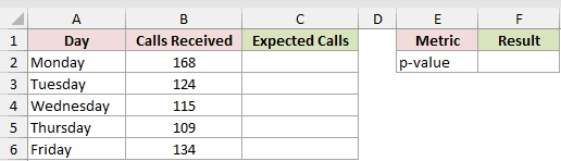
We want to calculate an equal expected count for each weekday, then test whether the observed calls follow that distribution.
Here is the formula:
=SUM($B$2:$B$6)/ROWS($B$2:$B$6)
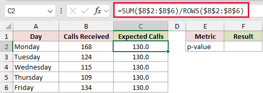
After filling the expected count through C6, here is the CHISQ.TEST formula:
=CHISQ.TEST(B2:B6,C2:C6)
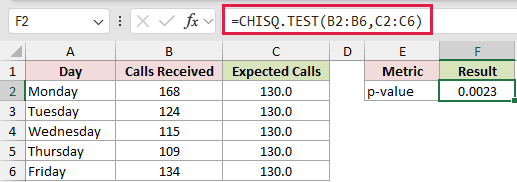
The first formula divides 650 total calls by five weekdays. It returns 130.0 in C2, and the same formula fills down through C6.
CHISQ.TEST compares the five observed counts with those five expected counts. A single column with five categories gives four degrees of freedom.
The p-value is 0.0023, which is below 0.05. The result is statistically significant, so the weekday call counts are not evenly distributed.
Example 2: Compare Orders With Benchmark Shares
Here’s a practical benchmark comparison.
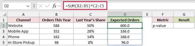
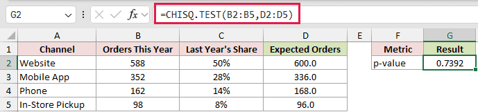
Below is the dataset with order channels, this year’s counts, and last year’s shares. Expected Orders has not been calculated yet, and the p-value cell is blank.

First, we’ll convert the historical shares into expected order counts, then test whether this year’s channel mix differs from that benchmark.
Here is the formula:
=SUM(B2:B5)*C2:C5
With the expected counts in place, use this formula:
=CHISQ.TEST(B2:B5,D2:D5)
How this formula works:
SUM(B2:B5)returns 1,200 orders, which the formula multiplies by the shares in C2:C5.- Entered in D2, the first formula spills 600.0, 336.0, 168.0, and 96.0 into D2:D5.
- CHISQ.TEST compares this year’s counts with those expected counts and returns 0.7392.
- At 0.7392, the p-value is above 0.05. The data does not show a statistically significant change in the channel mix, though it does not prove the mixes are identical.
Pro Tip: Never use the raw percentages in C2:C5 as the expected range. Convert them to counts first, or the chi-square statistic balloons to about 1.44 million.
Example 3: Chi-Square Test of Independence
Now let’s work with a two-way table.
Below is the dataset with regions, meal-kit choices, and helper totals. SUM formulas calculate the Total row and Total column.
The Expected table and p-value cell are blank.
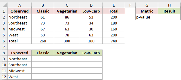
Next, we’ll calculate the expected counts and test whether meal-kit choice is associated with region.
Here is the formula:
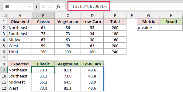
=E2:E5*B6:D6/E6
Then use this formula for the test:
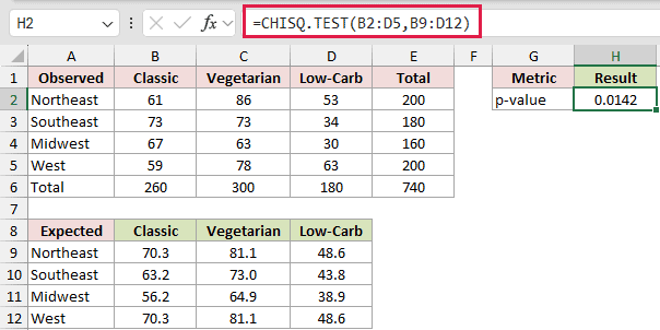
=CHISQ.TEST(B2:D5,B9:D12)
How this formula works:
E2:E5contains the row totals,B6:D6contains the column totals, and E6 contains the grand total.- The multiplication creates every row-and-column combination. Dividing by E6 returns the complete 4-by-3 expected table, with 70.3 as its first displayed value.
- CHISQ.TEST compares B2:D5 with B9:D12. Neither range includes the Total row or Total column.
- A 4-by-3 table gives six degrees of freedom. Its p-value is 0.0142. Against a 0.05 cutoff, the results indicate an association between region and meal-kit choice.
The totals-based formula works in Excel 2021, Excel 2024, and Microsoft 365. It creates the expected table with one spill.
Pro Tip: A common guideline is to use expected counts of at least 5. Check this table with =MIN(B9:D12). Its minimum is 38.92, and every example here meets that guideline.
Example 4: Calculate the Chi-Square Statistic
This example separates the p-value from the statistic behind it.
Below is the dataset with three landing-page versions, signup outcomes, and helper totals. SUM formulas calculate the Total row and Total column.
The Expected table and four Result cells are blank.
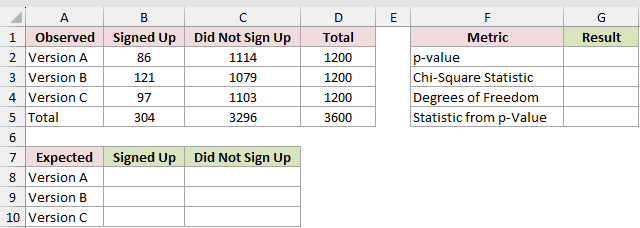
The goal is to calculate expected counts, return the p-value, report the chi-square statistic and degrees of freedom, then verify the statistic from the p-value.
Here is the formula:
=D2:D4*B5:C5/D5
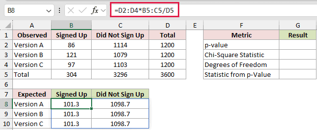
Here is the formula for the p-value:
=CHISQ.TEST(B2:C4,B8:C10)
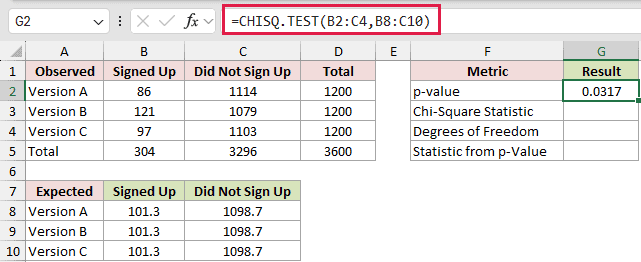
To calculate the chi-square statistic directly, use this formula:
=SUM((B2:C4-B8:C10)^2/B8:C10)
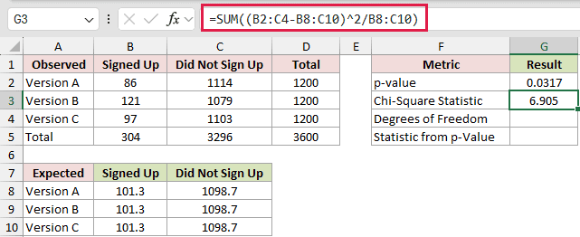
Here is the formula for the degrees of freedom:
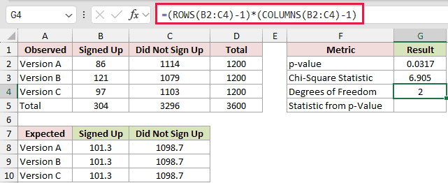
=(ROWS(B2:C4)-1)*(COLUMNS(B2:C4)-1)
Finally, use this formula to recover the statistic from the p-value:
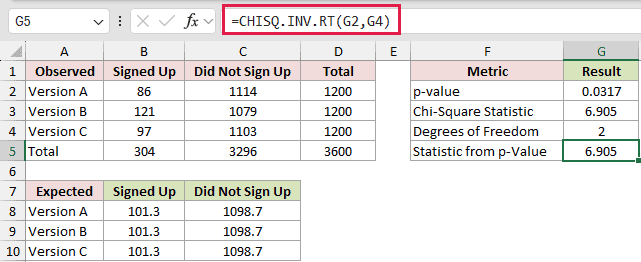
=CHISQ.INV.RT(G2,G4)
How these formulas work:
- The expected-count formula uses each row total, the two column totals, and the grand total. It spills into B8:C10, starting with 101.3.
- CHISQ.TEST returns 0.0317, the p-value. With a result below 0.05, the data supports an association between signup outcome and landing-page version.
SUM((B2:C4-B8:C10)^2/B8:C10)adds each squared observed-minus-expected difference divided by its expected count. It returns 6.905.- The ROWS and COLUMNS calculation returns two degrees of freedom for the 3-by-2 table.
- CHISQ.INV.RT uses the p-value in G2 and degrees of freedom in G4. It returns 6.905, confirming the directly calculated statistic.
The SUM array calculation works as a normal entry in Excel 2021 or later. In Excel 2019 and earlier, confirm it with Ctrl+Shift+Enter or use SUMPRODUCT.
If the statistic is already available, CHISQ.DIST.RT can take it with the degrees of freedom and return the same p-value.
Example 5: Chi-Square Test From Survey Data
Let’s finish with raw survey responses.
Below is the dataset with 40 age-group and preferred-channel responses. The Observed and Expected tables are blank, along with the p-value cell.
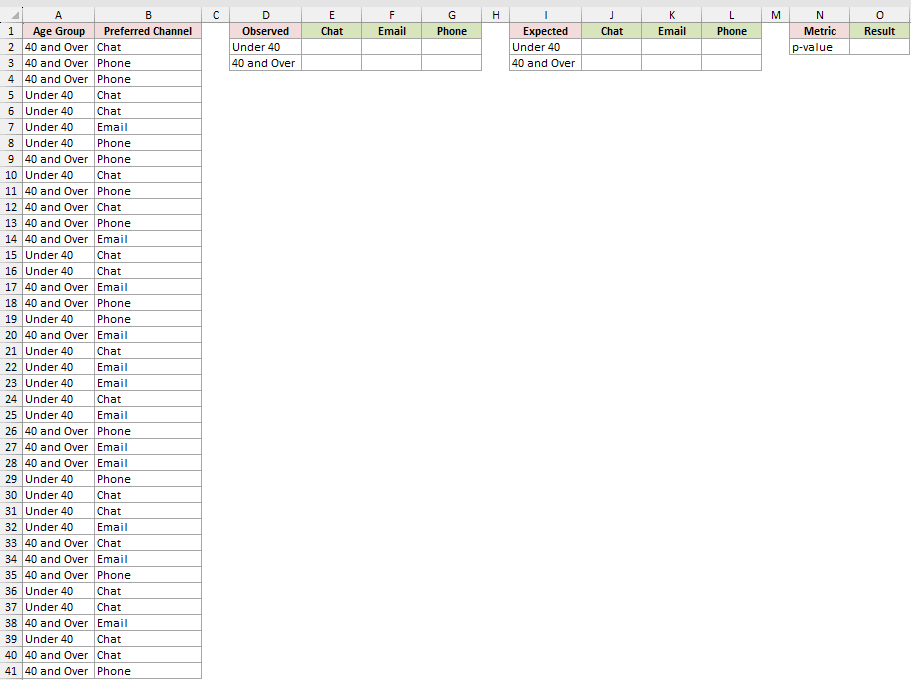
Here, we’ll build observed and expected crosstabs from the raw rows, then test whether preferred channel is associated with age group.
Here is the formula:
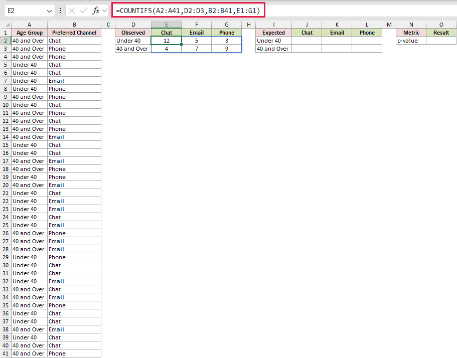
=COUNTIFS(A2:A41,D2:D3,B2:B41,E1:G1)
Next, calculate the expected crosstab with this formula:
=COUNTIF(A2:A41,I2:I3)*COUNTIF(B2:B41,J1:L1)/ROWS(A2:A41)
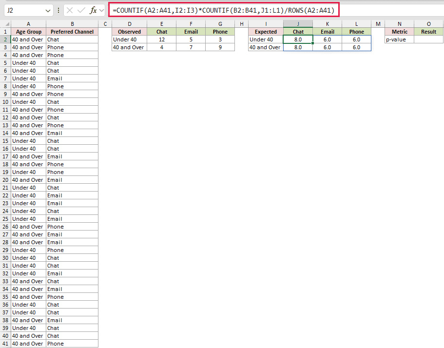
Then test the two spilled tables with this formula:
=CHISQ.TEST(E2#,J2#)
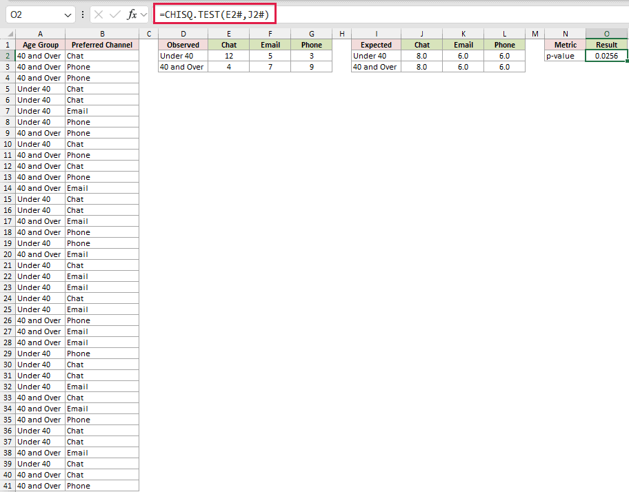
How these formulas work:
- COUNTIFS combines the age-group criteria in D2:D3 with the channel headers in E1:G1. The resulting 2-by-3 table spills from E2, starting with 12.
- The expected-count formula multiplies each age-group total by each channel total, then divides by 40 responses. It spills from J2, starting with 8.0.
- The
#operators make E2# and J2# refer to the complete spilled ranges. CHISQ.TEST then compares those complete tables. - CHISQ.TEST returns 0.0256. Compared with a 0.05 cutoff, this supports an association between age group and preferred channel.
These spills work in Excel 2021, Excel 2024, and Microsoft 365. Keep the cells around E2 and J2 empty so the tables can expand.
Tips & Common Mistakes
- Keep
actual_rangeandexpected_rangethe same shape. CHISQ.TEST returns#N/Awhen they contain different numbers of data points. - Exclude Total rows and Total columns from both ranges. Including totals can inflate the inferred degrees of freedom and produce the wrong p-value.
- Interpret the p-value against a chosen significance level, often 0.05. A large p-value does not prove that the observed and expected distributions are identical.
- Excel infers degrees of freedom from range shape. A table uses
(rows-1)*(columns-1), while a single row or column uses the number of categories minus one. - CHISQ.TEST returns one p-value rather than spilling. Supporting expected tables can spill in Excel 2021, Excel 2024, and Microsoft 365, so keep their spill areas clear.
- Excel applies no Yates continuity correction. Results for 2-by-2 tables can differ from SPSS or R when those programs apply the correction.
- CHISQ.DIST.RT returns the same p-value when you already have the chi-square statistic and degrees of freedom.
- CHISQ.TEST is available in Excel 2010 and later. It replaced CHITEST, which remains the older compatibility name.
I’ve shown how CHISQ.TEST returns a p-value from observed and expected counts, including tables built from totals, benchmarks, and raw responses.
I also covered calculating the chi-square statistic and degrees of freedom alongside the test.
I hope you found this article helpful.
Related Excel Functions / Articles:
