
Excel’s T.TEST function returns the p-value associated with a Student’s t-test for two sets of observations.
You choose a one-tailed or two-tailed test and specify whether the data are paired or independent. Those choices need to match the comparison you are making.
The result is a p-value, not the t statistic, the size of the difference, or an indication of which group is larger.
In this article, I’ll show you how to run paired comparisons, choose one or two tails, and compare the three available test types.
T.TEST Function Syntax in Excel
The T.TEST function compares two sets of numeric values and returns their p-value.
=T.TEST(array1,array2,tails,type)
- array1 (required) is the first set of numeric values.
- array2 (required) is the second set of numeric values.
- tails (required) is 1 for a one-tailed test or 2 for a two-tailed test.
- type (required) is 1 for paired data, 2 for independent groups with equal variance, or 3 for independent groups with unequal variance.
The p-value guide and calculator explain the statistical concept itself. T.TEST returns the p-value, while its tails and type arguments determine how Excel calculates it.
When to Use T.TEST Function
- Compare before and after measurements from the same people, machines, or campaigns.
- Compare two independent groups whose values may have equal or unequal variance.
- Test groups stored in a long-format table by building arrays with FILTER.
- Check several variants against one control and label the results.
- Compare one-tailed and two-tailed results after choosing the direction in advance.
Example 1: Run a Paired T.TEST
Let’s start with the case where every before value has a matching after value.
Below is the dataset. Column A lists ten agents, while columns B and C contain each agent’s before and after handle times.
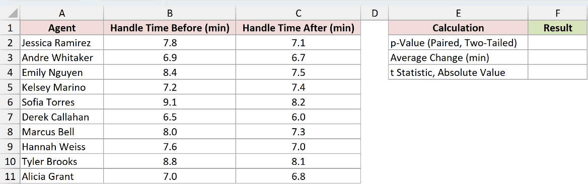
We want the two-tailed p-value for the change in handle time across these matched agents.
Here is the paired T.TEST formula:
=T.TEST($B$2:$B$11,$C$2:$C$11,2,1)
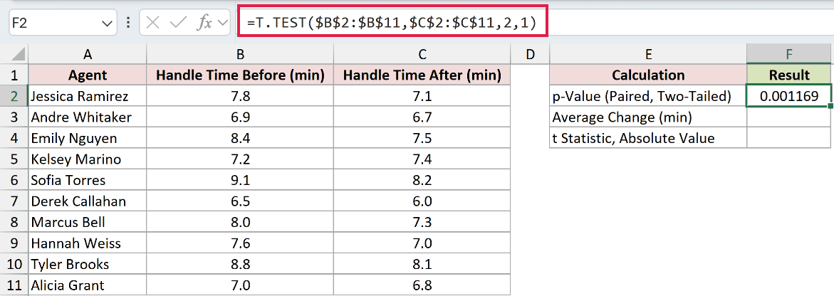
The formula returns 0.001169. The final argument is 1 because each row belongs to the same agent before and after the new script.
That p-value doesn’t show whether handle time rose or fell, so the next formula compares the two averages.
=AVERAGE($C$2:$C$11)-AVERAGE($B$2:$B$11)
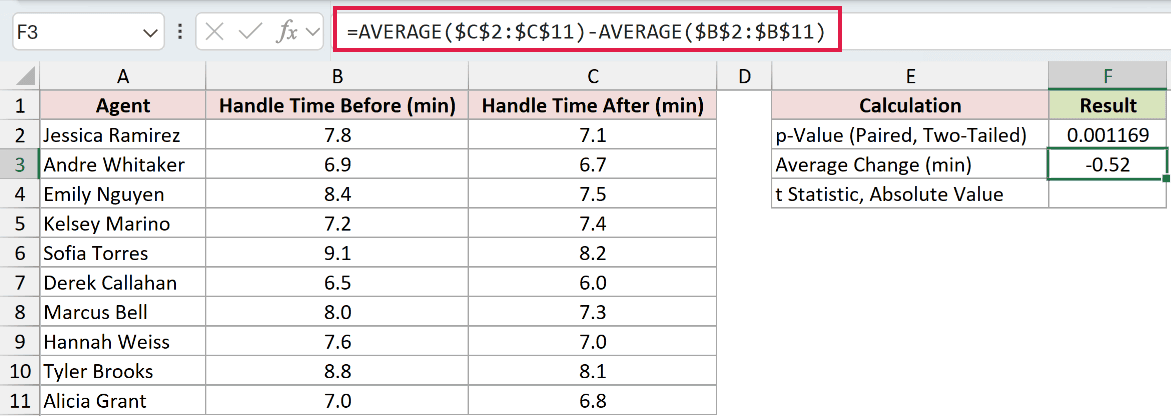
The result is -0.52 minutes. The negative sign shows the after average is lower, which supplies the direction T.TEST leaves out.
To recover the absolute t statistic, feed the p-value in F2 and the paired degrees of freedom into T.INV.2T.
=T.INV.2T(F2,COUNT($B$2:$B$11)-1)
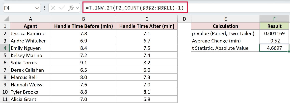
The formula returns 4.6697. T.INV.2T always returns a positive value, so use the average change to determine direction.
The Analysis ToolPak can return the statistic and other details in a static block. The p-value guide walks through that route.
Pro Tip: This recovery is exact for the paired test because it uses n minus 1 degrees of freedom. Type 3 is approximate because T.INV.2T truncates fractional degrees of freedom.
Example 2: Use T.TEST With FILTER
Here’s a practical way to test two groups stored in one column.
Below is the dataset. Column A contains visit IDs, column B identifies the lane type, and column C records checkout time in seconds.
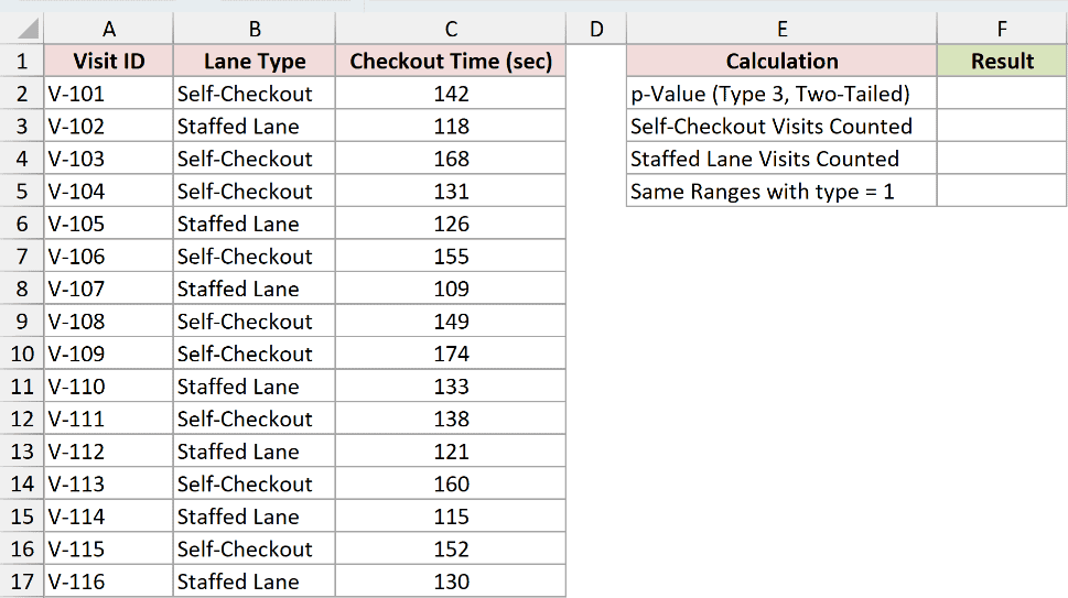
We want to compare self-checkout and staffed-lane times without copying either group into a helper column.
Here is the formula:
=T.TEST(FILTER($C$2:$C$17,$B$2:$B$17="Self-Checkout"),FILTER($C$2:$C$17,$B$2:$B$17="Staffed Lane"),2,3)
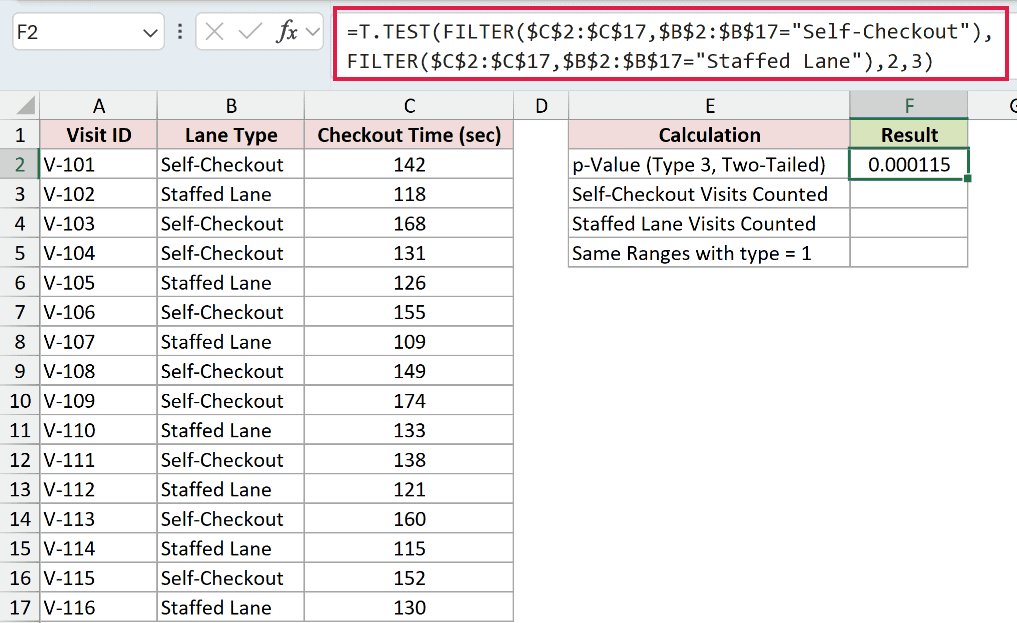
Each FILTER call creates one input array from column C. T.TEST then reduces those arrays to the p-value 0.000115.
The first COUNTIF checks how many self-checkout visits entered the test.
=COUNTIF($B$2:$B$17,"Self-Checkout")
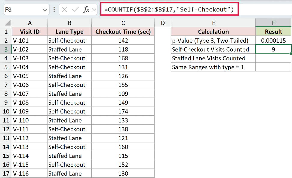
The result is 9.
The second COUNTIF counts the staffed-lane visits.
=COUNTIF($B$2:$B$17,"Staffed Lane")
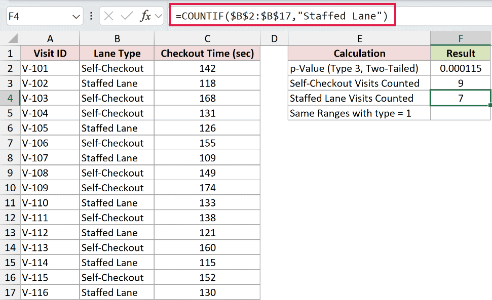
That result is 7. Types 2 and 3 can compare independent groups with different sample sizes.
The same arrays produce an error when they are incorrectly treated as paired data.
=T.TEST(FILTER($C$2:$C$17,$B$2:$B$17="Self-Checkout"),FILTER($C$2:$C$17,$B$2:$B$17="Staffed Lane"),2,1)
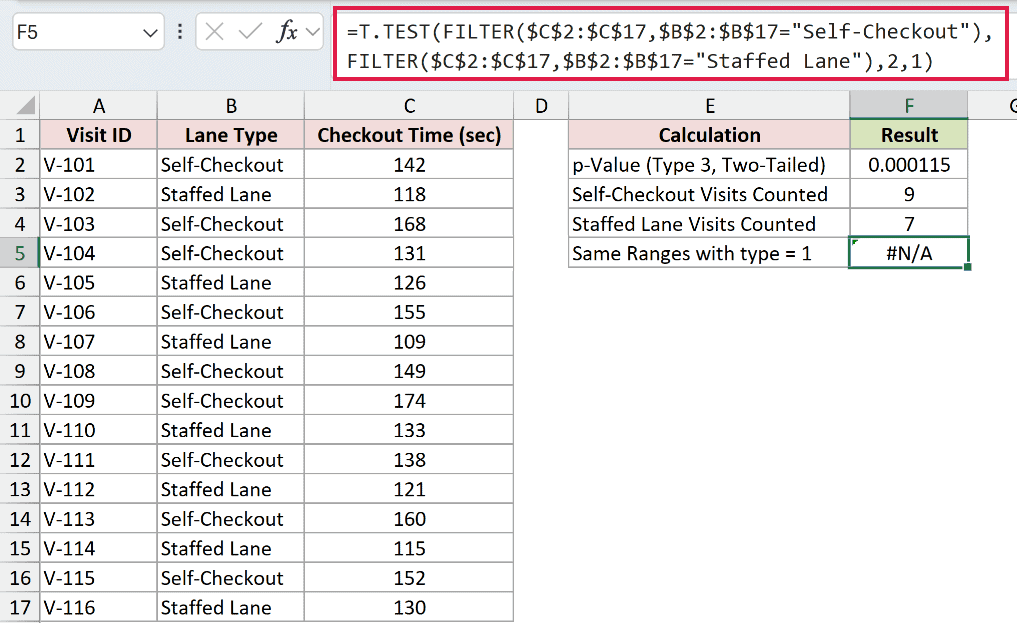
The formula returns #N/A because type 1 needs equal-length arrays whose rows form genuine pairs.
Pro Tip: FILTER requires Excel 2021, Excel 2024, Microsoft 365, or Excel for the web. Excel 2019 and earlier return #NAME?, so sort or copy each group into a separate range.
Example 3: Compare All Three T.TEST Types
This example shows why the type argument isn’t a setting to guess at.
Below is the dataset. Column A identifies twelve ad sets, while columns B and C contain each set’s search and social cost per click.
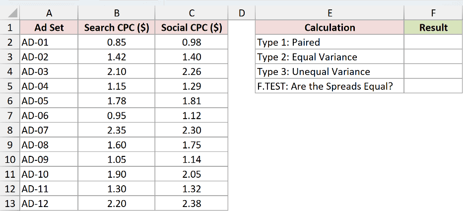
We want to run all three test types on the same ranges and compare their answers.
First, here is the paired test:
=T.TEST($B$2:$B$13,$C$2:$C$13,2,1)
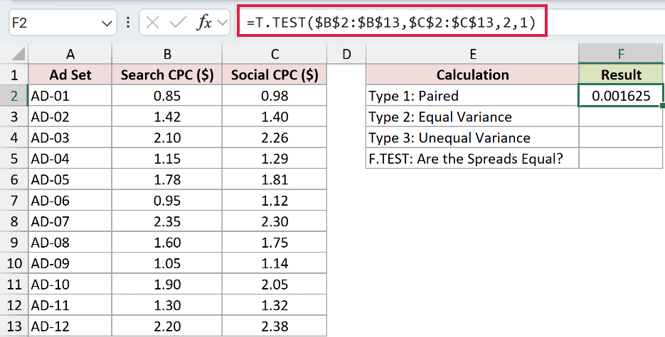
Type 1 returns 0.001625. It fits this setup because each search value and social value belong to the same ad set.
Next, here is the equal-variance test for independent groups:
=T.TEST($B$2:$B$13,$C$2:$C$13,2,2)
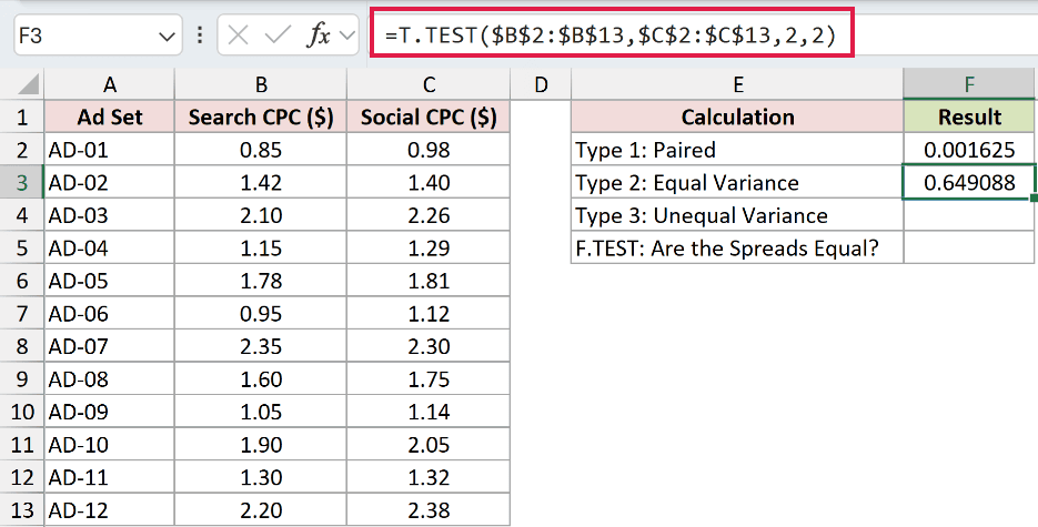
Type 2 returns 0.649088.
And here is Welch’s unequal-variance test for independent groups:
=T.TEST($B$2:$B$13,$C$2:$C$13,2,3)
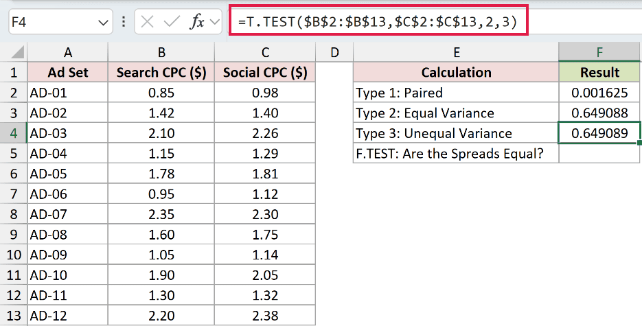
Type 3 returns 0.649089. Types 2 and 3 are nearly identical here, but both are far from the paired result.
Here is the one F.TEST check used to compare the two spreads:
=F.TEST($B$2:$B$13,$C$2:$C$13)
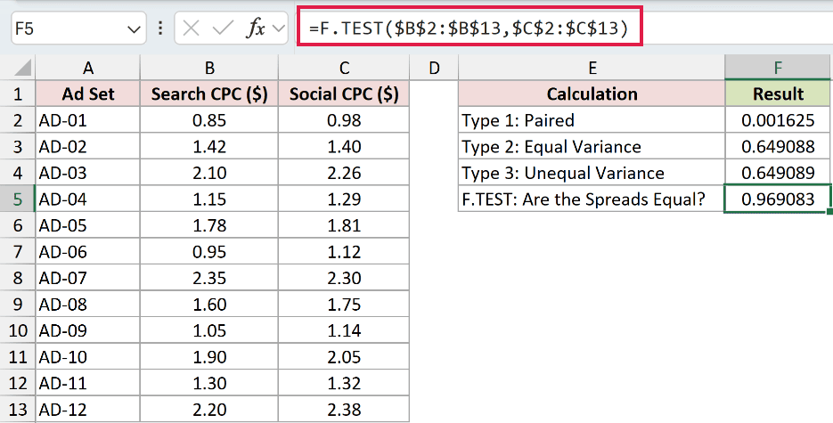
Its 0.969083 result says the spreads are similar. That explains why types 2 and 3 differ only in the sixth decimal.
If you are unsure whether the spreads match, type 3 is the safer choice. It costs almost nothing when they do match.
The bigger decision is paired versus independent. Base that choice on how the data was collected.
Example 4: Choose One Tail or Two
Now let’s see why the tails argument must be chosen before you inspect the answer.
Below is the dataset. Columns A and B contain one shipment batch, while columns C and D contain a separate batch from the new carrier.
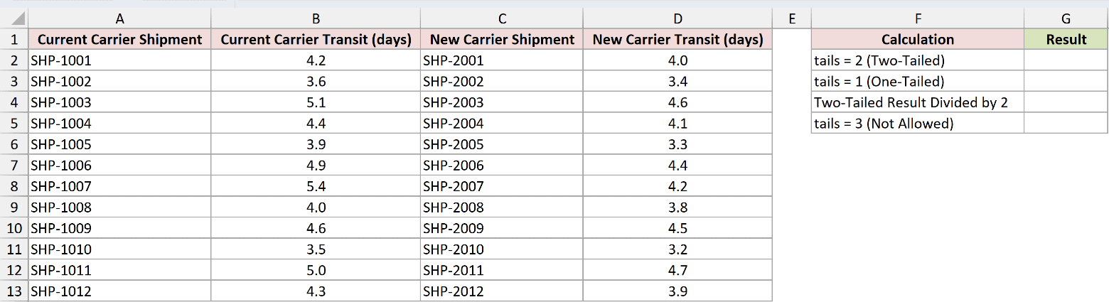
We want to compare two-tailed and one-tailed results using the unequal-variance test.
Here is the two-tailed formula:
=T.TEST($B$2:$B$13,$D$2:$D$13,2,3)
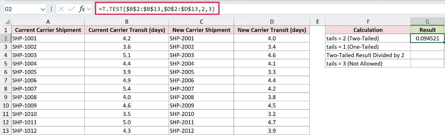
The formula returns 0.094521.
Here is the one-tailed version:
=T.TEST($B$2:$B$13,$D$2:$D$13,1,3)
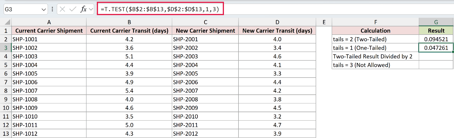
The result is 0.047261, exactly half the two-tailed value.
The next formula makes that relationship visible.
=G2/2
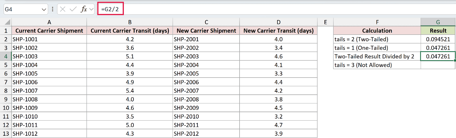
Dividing 0.094521 by 2 also displays 0.047261.
Excel’s one-tailed result is direction-blind. Swapping the two input ranges returns the same value, so the function doesn’t tell you which carrier is faster.
If the observed difference runs against your stated direction, the relevant one-tailed probability is one minus Excel’s returned value.
Finally, here is an invalid tails value:
=T.TEST($B$2:$B$13,$D$2:$D$13,3,3)
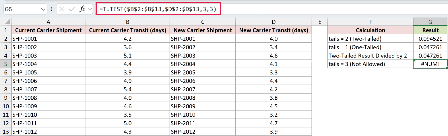
The formula returns #NUM! because tails accepts only 1 or 2.
Pro Tip: Choose a one-tailed test before looking at the data. Switching from two tails after seeing 0.094521 is p-hacking and undermines the analysis.
Example 5: Screen Variants Against a Control
Finally, let’s compare several independent variants with one current design.
Below is the dataset. Columns A through D hold four independent signup runs: Current 12, Variant A 11, Variant B 12, and Variant C 10.
They aren’t matched rows with missing data.
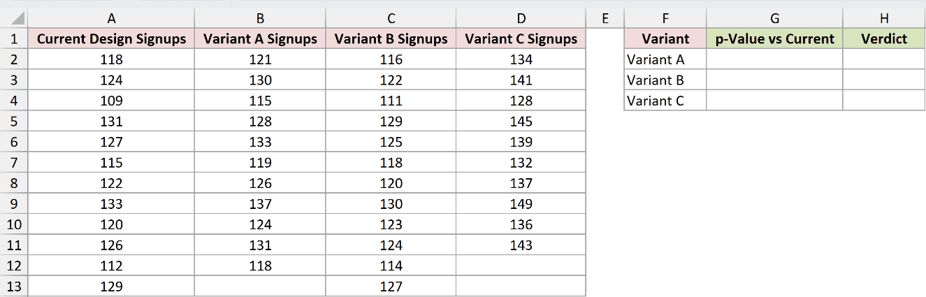
We want a p-value and a plain-language verdict for every variant.
Here is the T.TEST formula for Variant A:
=T.TEST($A$2:$A$13,$B$2:$B$12,2,3)
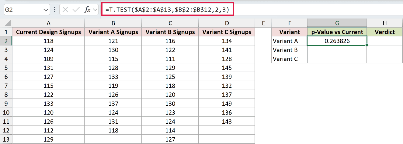
The formula returns 0.263826.
This IF formula turns that p-value into the worksheet’s verdict:
=IF(G2<0.05,"Significant","No clear difference")
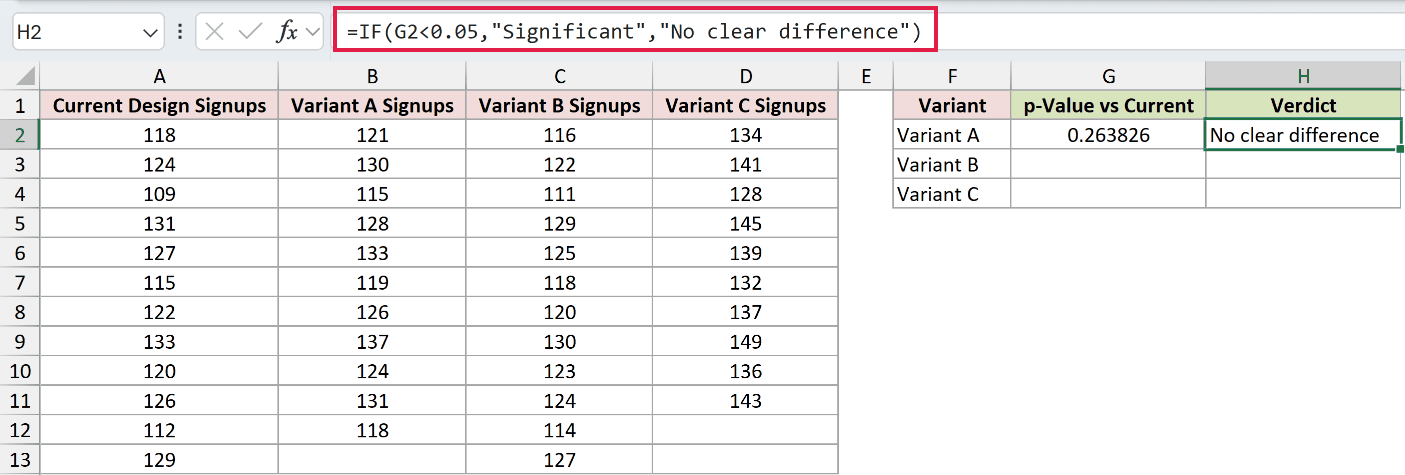
Variant A is labeled No clear difference.
Here is the T.TEST formula for Variant B:
=T.TEST($A$2:$A$13,$C$2:$C$13,2,3)
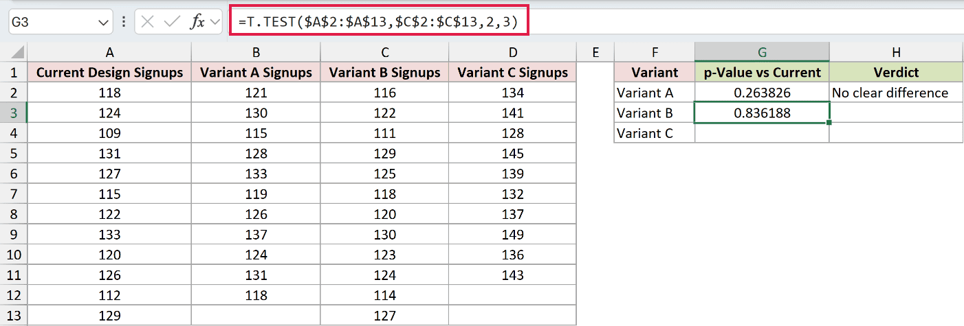
The formula returns 0.836188.
And here is the matching verdict formula:
=IF(G3<0.05,"Significant","No clear difference")
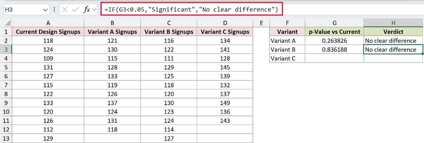
Variant B is also labeled No clear difference.
Here is the T.TEST formula for Variant C:
=T.TEST($A$2:$A$13,$D$2:$D$11,2,3)
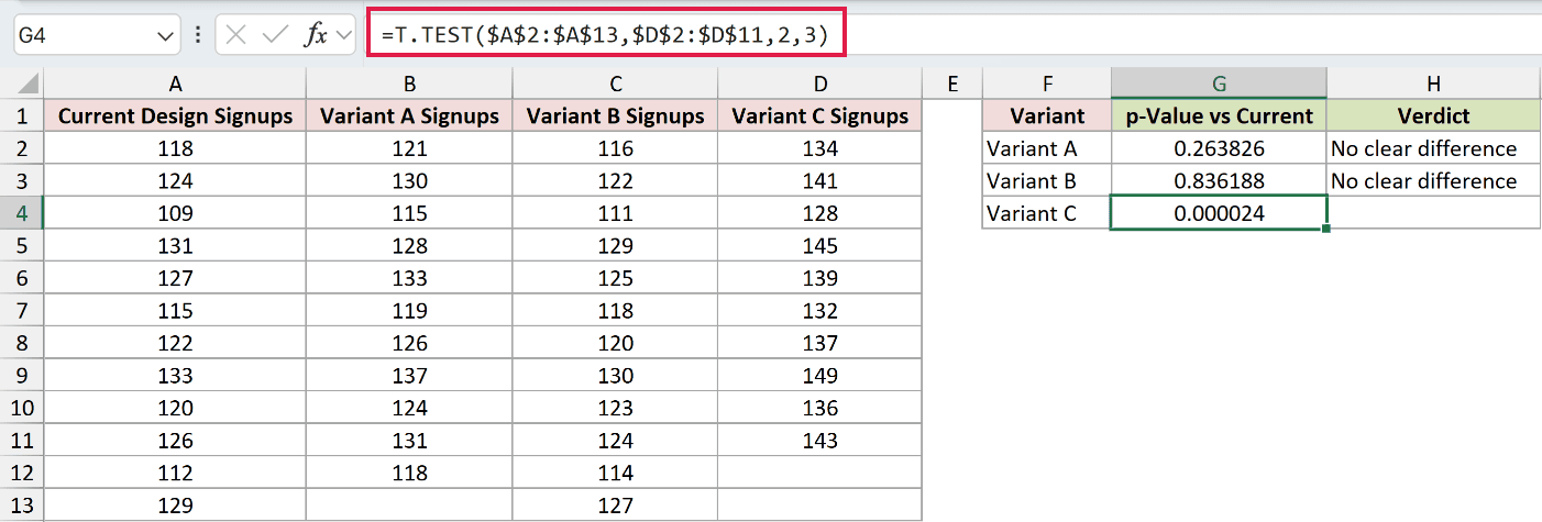
The formula returns 0.000024. The cell displays six decimal places, while Excel keeps the underlying precision.
Here is the final verdict formula:
=IF(G4<0.05,"Significant","No clear difference")
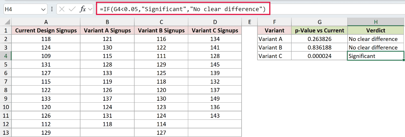
Variant C is labeled Significant.
Running several tests against one control increases the chance that one result looks significant by luck. Treat this screen as an initial check that needs further evidence.
Tips & Common Mistakes
- T.TEST returns one p-value. It doesn’t return the t statistic, degrees of freedom, group averages, effect size, or direction.
- Use type 1 only for genuine matched pairs. Use type 2 for independent groups with equal variance and type 3 for independent groups with unequal variance.
tailsaccepts only 1 or 2, whiletypeaccepts only 1, 2, or 3. Values outside those sets after truncation return #NUM!, and nonnumeric values return #VALUE!.- Excel truncates decimal
tailsandtypevalues to integers, sotailsof 2.9 quietly behaves as 2. - T.TEST accepts spilled range references such as
A2#, but it still reduces the two arrays to one p-value. - The older TTEST name still works and returns the same value. T.TEST is the current name to use in new workbooks.
- A small p-value doesn’t tell you whether a change is large or useful. Example 1 pairs 0.001169 with an average change of -0.52 minutes for that reason.
T.TEST returns one probability. Choose tails and type before reading the result.
Use the collection method to choose the type, and compare the group averages when you need direction or practical size.
Related Excel Functions / Articles:
