
The COVARIANCE.P function in Excel returns the population covariance between two sets of values.
It shows whether paired values tend to move together. A positive result means they generally rise together, while a negative result means they tend to move in opposite directions.
Use it when your rows represent the complete population you want to analyze, rather than a sample taken from a larger group.
In this article, I’ll show you how to compare population and sample covariance, handle incomplete or imported data, and turn covariance into a scale-free correlation.
COVARIANCE.P Function Syntax in Excel
COVARIANCE.P takes two equally sized arrays containing the paired values.
=COVARIANCE.P(array1, array2)
- array1 (required) is the first range or array of numeric values.
- array2 (required) is the second range or array of numeric values paired by position with array1.
Excel ignores text, logical values, and empty cells in references. If either value in a pair is ignored, Excel drops that whole pair. Zeros remain part of the calculation.
When to Use COVARIANCE.P Function
- Check whether two measures move together across every member of a complete group.
- Compare operational measures such as activity and cost across a finished reporting period.
- Normalize covariance with population standard deviations when you need a correlation.
- Analyze one complete subgroup by passing filtered arrays to COVARIANCE.P.
Example 1: Population Covariance for Every Store
Let’s start with a complete group rather than a sample.
Below is the dataset. All seven stores in the chain appear with Loyalty Members and Monthly Sales, plus a labeled empty cell for population covariance.
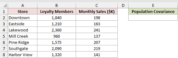
We want to measure how loyalty membership and monthly sales move together across the whole chain.
Here is the formula:
=COVARIANCE.P(B2:B8,C2:C8)
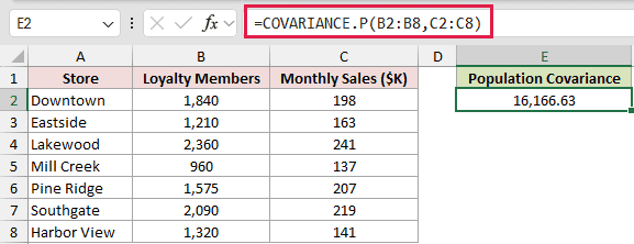
The formula returns 16,166.63. Its positive sign shows that stores with more loyalty members generally also have higher monthly sales.
The magnitude depends on the scales and units of both columns. It doesn’t work like a standardized score, so compare the sign before judging the size.
Example 2: COVARIANCE.P vs COVARIANCE.S
Now let’s compare the population and sample versions on the same finished year.
Below is the dataset. The sheet covers every month, with Oven Hours, Electric Bill, and labeled empty cells for both covariance measures and the manual check.
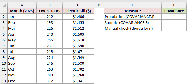
We want population covariance because the data covers the complete year being analyzed.
Here is the COVARIANCE.P formula:
=COVARIANCE.P(B2:B13,C2:C13)
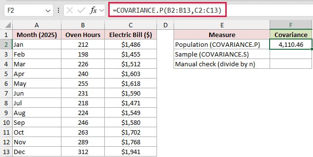
The population formula returns 4,110.46.
Here is the COVARIANCE.S formula for comparison:
=COVARIANCE.S(B2:B13,C2:C13)
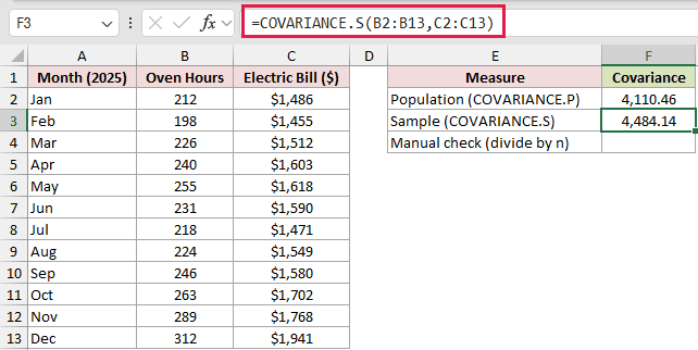
The sample comparison returns 4,484.14. Here the covariance is positive, so it is larger than the population result of 4,110.46.
COVARIANCE.S divides by one fewer observation, or n-1. For these 12 months, 4,484.14 = 4,110.46 x 12/11.
Here is the manual population calculation:
=SUMPRODUCT((B2:B13-AVERAGE(B2:B13))*(C2:C13-AVERAGE(C2:C13)))/COUNT(B2:B13)
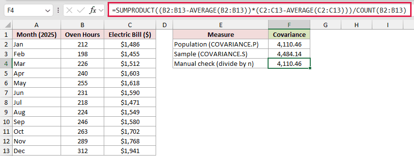
The manual check also returns 4,110.46. It subtracts each column’s average, multiplies the paired deviations, totals them, and divides by the population count.
Pro Tip: Use COVARIANCE.P when the rows are the complete group you care about. Use COVARIANCE.S when those rows are a sample from a larger population.
Example 3: Convert Covariance to Correlation
Covariance shows direction, but its size changes with the units in your columns.
Below is the dataset. Each fleet truck appears with Age and Annual Repair Cost, followed by labeled empty cells for covariance and two correlation checks.
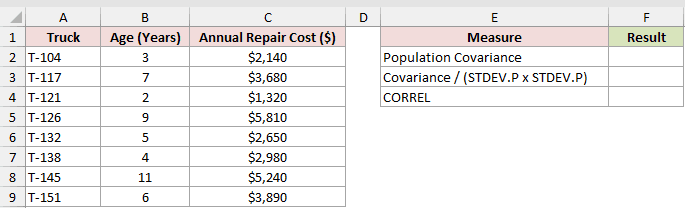
We first want the population covariance between truck age and annual repair cost.
Here is the formula:
=COVARIANCE.P(B2:B9,C2:C9)
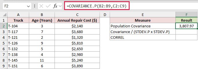
The formula returns 3,807.97. Its unit is years multiplied by dollars, which makes the size difficult to interpret by itself.
We can divide by both population standard deviations to remove those units:
=COVARIANCE.P(B2:B9,C2:C9)/(STDEV.P(B2:B9)*STDEV.P(C2:C9))
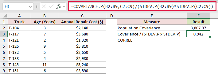
The normalized result is 0.942. Pair population covariance with STDEV.P for both columns so the calculation uses population measures consistently.
Here is CORREL as the direct comparison:
=CORREL(B2:B9,C2:C9)
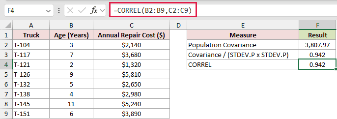
CORREL also returns 0.942. Use it when you want the scale-free relationship directly rather than the original covariance units.
Example 4: Handle Blank and Text Pairs
Incomplete rows are easy to misread because COVARIANCE.P can skip them without returning an error.
Below is the dataset. The branch table pairs Open Hours per Week with Weekly Checkouts. One input is blank, another is text, and the answer sits above the +0 mistake.
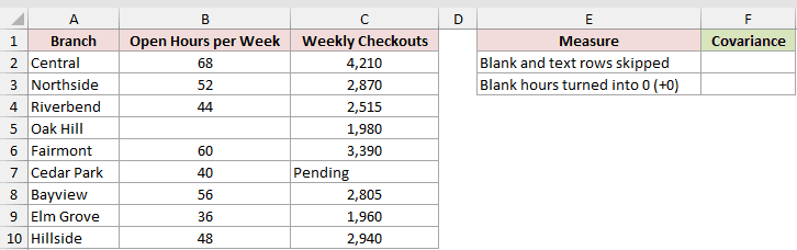
We want covariance from the complete numeric pairs while leaving the incomplete rows out.
Here is the formula:
=COVARIANCE.P(B2:B10,C2:C10)
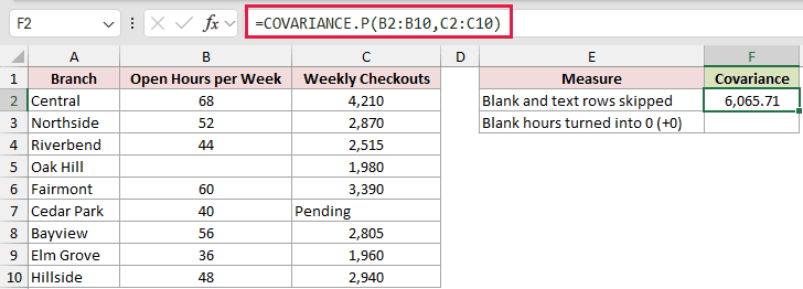
The formula returns 6,065.71. Excel drops Oak Hill’s whole pair because its hours cell is blank, and it drops Cedar Park’s pair because checkouts contains text.
Here is the wrong way to coerce the hours range:
=COVARIANCE.P(B2:B10+0,C2:C10)
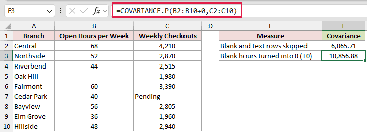
This mistake returns 10,856.88. Adding zero turns Oak Hill’s blank into a real zero, inventing a pair that wasn’t present in the source data.
Pro Tip: Don’t use +0 to clean a covariance range containing genuine blanks. It changes which pairs Excel includes and can silently change the answer.
Example 5: Fix Numbers Stored as Text
Imported data creates the opposite problem when valid numbers arrive as text.
Below is the dataset. Its three input columns are Building, Apartments, and Maintenance Requests.
Cedar Court’s 39, Oakmont’s 40, and Parkside’s 17 are numbers stored as text. Their left alignment is the visible clue despite the 0 format.
The As imported and Text converted with -- labels sit beside empty Covariance cells.
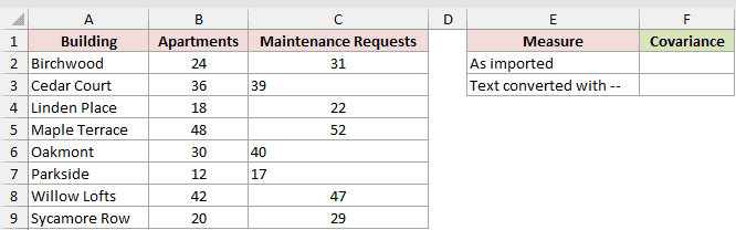
We first want to see the silent wrong answer returned from the data as imported.
Here is the as-imported formula:
=COVARIANCE.P(B2:B9,C2:C9)
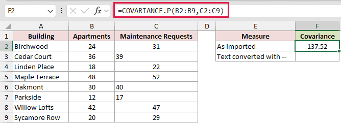
The as-imported result is 137.52, but it is wrong. Excel skips the rows where maintenance requests are numbers stored as text.
Here is the corrected formula using the double unary operator:
=COVARIANCE.P(B2:B9,--C2:C9)
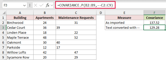
The corrected formula returns 129.28. The double unary operator converts the text numbers before COVARIANCE.P evaluates the pairs.
Pro Tip: The -- fix is safe here because the column has no genuine blanks. Clean the source data instead when blanks and text numbers may appear together.
Example 6: Covariance for Filtered Data
COVARIANCE.P returns one value, but it can reduce arrays created by dynamic array functions.
Below is the dataset. Machines are grouped by Line alongside Hours Since Service and Scrap Parts. A selected Line and a labeled empty covariance cell complete the sheet.
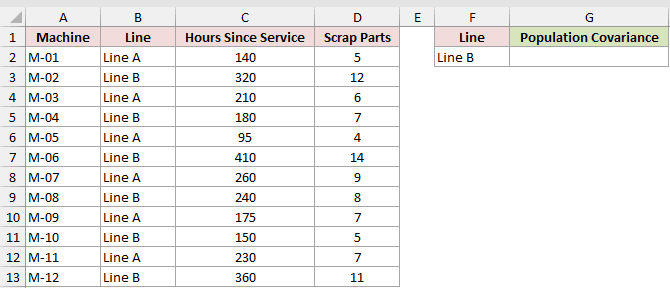
We want population covariance for Line B without building helper columns.
Here is the formula:
=COVARIANCE.P(FILTER(C2:C13,B2:B13=F2),FILTER(D2:D13,B2:B13=F2))
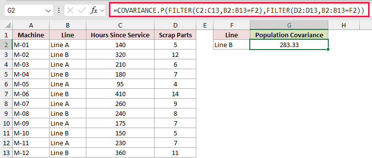
Each FILTER returns the Line B values from one measure. COVARIANCE.P then reduces those paired arrays to 283.33.
FILTER needs Excel 2021 or later. COVARIANCE.P itself is available in Excel 2010 and later.
Pro Tip: If FILTER finds no matching rows, it returns #CALC!, and that error passes through COVARIANCE.P. Check the criterion when a group is missing.
Tips & Common Mistakes
- COVARIANCE.P is a reducer. It accepts two arrays but returns one covariance value rather than spilling a result for every row.
- Legacy COVAR returns the same population covariance as COVARIANCE.P. Don’t replace it with COVARIANCE.S unless the data is genuinely a sample.
- Unequal range sizes return #N/A. A column and a row can still be paired when they contain the same number of values because Excel pairs by position.
- One numeric pair returns 0 with COVARIANCE.P, while COVARIANCE.S returns #DIV/0!. That population result doesn’t prove there is no relationship.
- If no numeric pairs remain, COVARIANCE.P returns #DIV/0!. Errors already present in either input range pass through the formula.
- Adding a constant to one variable doesn’t change covariance. Multiplying a variable scales it, and reversing one variable’s sign reverses the covariance sign.
- A variable’s covariance with itself equals its population variance. Use VAR.P when that is the value you need.
- A covariance matrix is a separate task for comparing several variables at once.
Before choosing the function, decide whether your rows truly cover the complete group you care about.
That one check keeps a population calculation from quietly becoming a sample calculation.
Related Excel Functions / Articles:
