How to Create a Covariance Matrix in Excel (3 Easy Ways)

If you want to see how several stocks or variables move together, a single covariance figure between two of them won’t tell the whole story. You need every pair at once, laid out in a grid.

That grid is a covariance matrix. Excel doesn’t have one obvious button for it, so it can feel harder to build than it really is.

The good news is there are a few reliable ways to get there. In this guide I’ll show you three: the Data Analysis ToolPak, the COVARIANCE.P function, and a single MMULT array formula.

If you only care about two variables rather than a full grid, how to calculate covariance in Excel walks through the single-pair version.

Table of Contents

Method #1: Using the Data Analysis ToolPak

This is the method I reach for first because it builds the entire matrix in one action, no formulas required. It’s the fastest route when you just want the numbers.

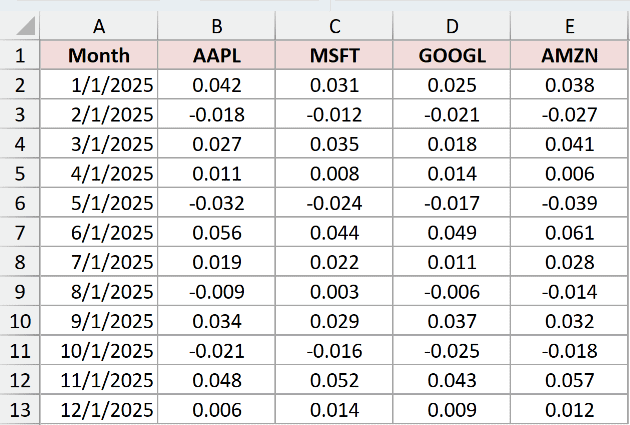
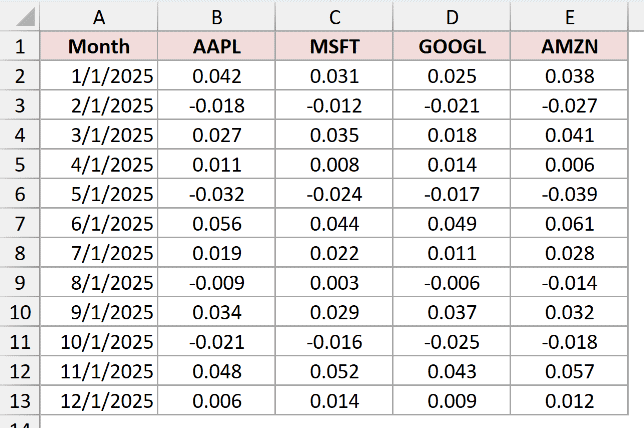
Below I have monthly returns for four stocks, AAPL, MSFT, GOOGL, and AMZN, across twelve months. The Month sits in column A, and each stock’s return runs down columns B to E.

Twelve months of returns for AAPL, MSFT, GOOGL and AMZN, with the month in column A

The ToolPak is an add-in, so it may not be switched on yet. If you don’t see a Data Analysis button on the Data tab, turn it on first.

Go to File, then Options, then Add-ins. At the bottom, next to Manage Excel Add-ins, click Go, tick Analysis ToolPak, and click OK.

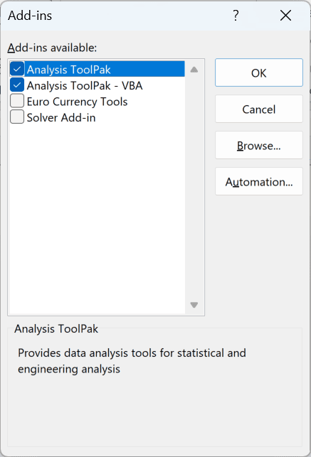
The Add-ins dialog reached through File, Options, Add-ins, where Analysis ToolPak is ticked

Once it’s enabled, here are the steps to build the covariance matrix:

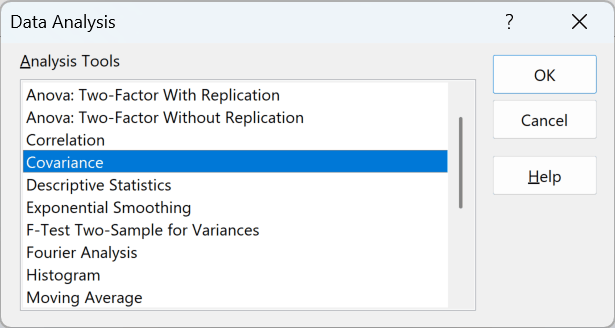
On the Data tab, click Data Analysis, choose Covariance from the list, and click OK.

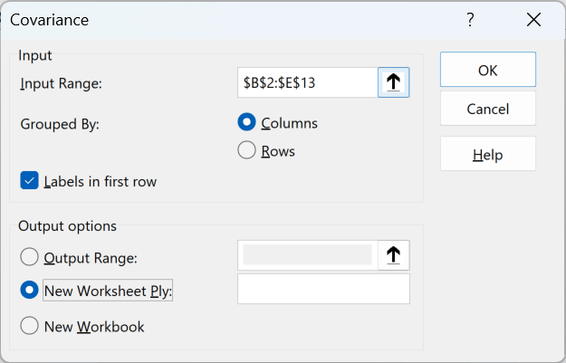
Excel Data Analysis dialog box with Covariance selected in the Analysis Tools list and buttons for OK, Cancel, and Help

Set the Input Range to B1:E13, choose Grouped By Columns, tick Labels in First Row, pick an Output Range for the result, and click OK.

Covariance dialog box with Input Range set to $B$2:$E$13, Columns selected, and Labels in first row checked

Excel drops a labeled grid into your output range. Each cell is the covariance between the stock on its row and the stock on its column.

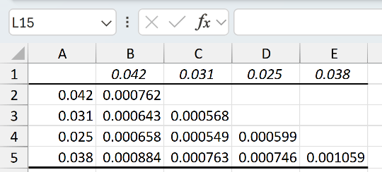
Excel spreadsheet showing a lower triangular covariance matrix with numerical values for five variables

Notice that only the lower-left triangle is filled. That’s on purpose. The covariance of AAPL with MSFT is the same as MSFT with AAPL, so Excel skips the mirror half.

The diagonal running top-left to bottom-right holds something special. Each of those cells is the stock’s covariance with itself, which is simply its variance.

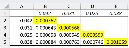
Spreadsheet showing a covariance matrix with the diagonal cells highlighted in yellow to show variance with itself

Note: The ToolPak output is static. It won’t recalculate if you edit the returns later, so re-run the tool after any change. It also uses population covariance (it divides by the number of months). The two formula methods below update live.

Method #2: Using the COVARIANCE.P Function

If you’d rather have a live matrix that recalculates on its own, build it with COVARIANCE.P. One formula, copied across a grid, gives you full control and updates the moment the data changes.

Here’s the same returns table, AAPL, MSFT, GOOGL, and AMZN down columns B to E, with the tickers as headers in row 1.

The same returns table with the tickers as headers in row 1 and returns running down columns B to E

First, set up an empty grid. Put the four tickers as row labels in G2:G5 and the same four as column labels in H1:K1. This frame tells the formula which two stocks each cell should compare.

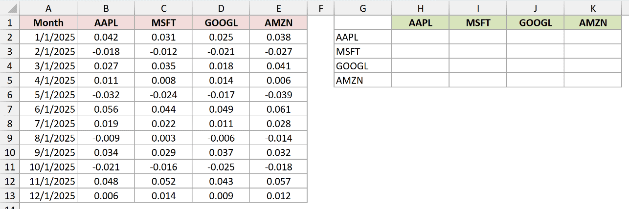
The empty matrix frame with the four tickers as row labels in G2 to G5 and the same four as column labels in H1 to K1

Here is the formula. Enter it in H2, then copy it across the whole grid, H2 to K5:

=COVARIANCE.P(INDEX($B$2:$E$13,0,MATCH($G2,$B$1:$E$1,0)),INDEX($B$2:$E$13,0,MATCH(H$1,$B$1:$E$1,0)))

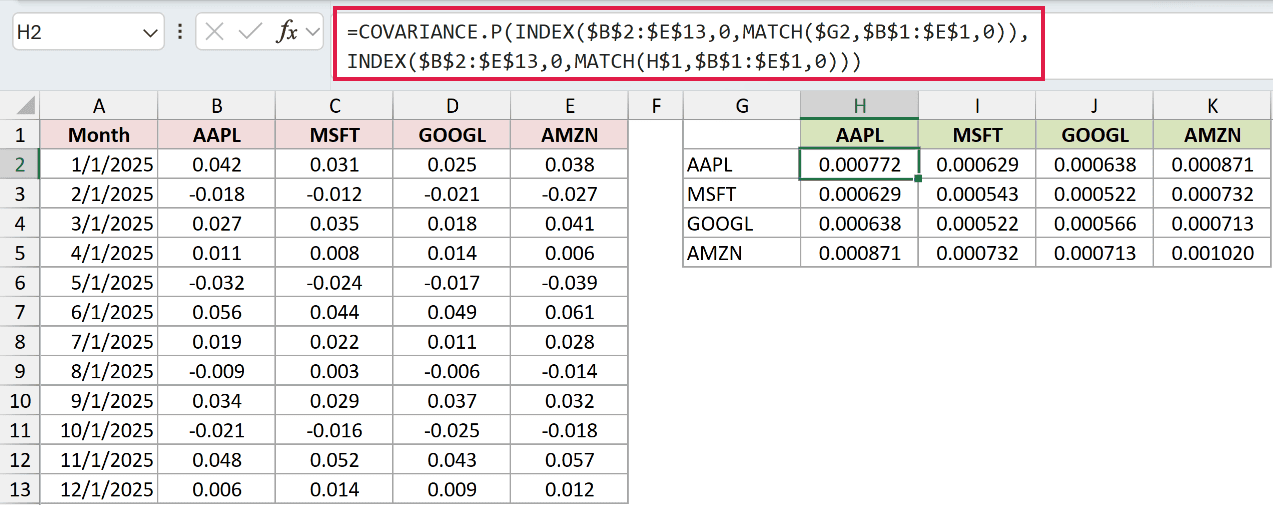
The COVARIANCE.P formula in cell H2 returning 0.000772 as AAPL's covariance with itself

Every cell fills in, and the numbers match the ToolPak matrix from Method #1.

How does this formula work?

MATCH($G2,$B$1:$E$1,0) looks at the row label in column G and finds which data column that ticker sits in. MATCH(H$1,$B$1:$E$1,0) does the same for the column label in row 1.

INDEX($B$2:$E$13,0,...) uses a row number of 0, which tells INDEX to return the entire column, not a single cell. So each INDEX hands back one full column of returns.

COVARIANCE.P then takes those two twelve-value columns and returns their covariance. The mixed references, $G2 and H$1, lock the label lookups so the one formula works in every cell of the grid.

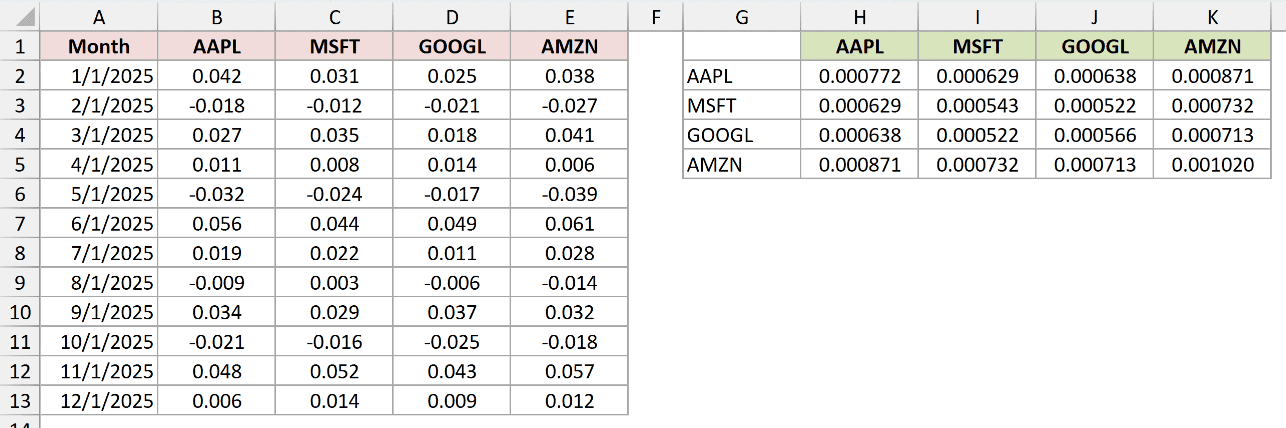
The finished four by four matrix, symmetric about a diagonal of 0.000772, 0.000543, 0.000566 and 0.001020

Because it fills the full square, you get both triangles, not just the lower half. The diagonal, where a stock meets itself, is its variance.

Note: COVARIANCE.P treats your rows as the whole population. If your twelve months are a sample of a longer history, swap in COVARIANCE.S, which divides by one less than the count.

Method #3: Using an MMULT Array Formula

For the shortest route in modern Excel, you can spill the entire matrix from a single formula using matrix multiplication. It’s the most advanced of the three, but once you see the pattern it’s compact.

Same returns table, four stocks in columns B to E over twelve months.

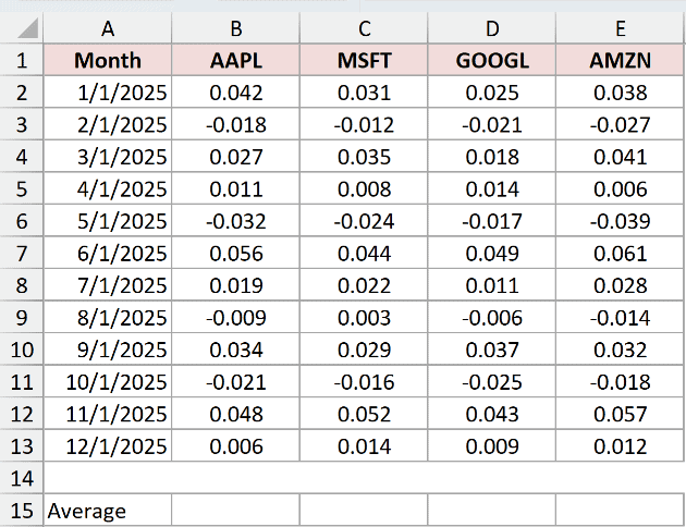
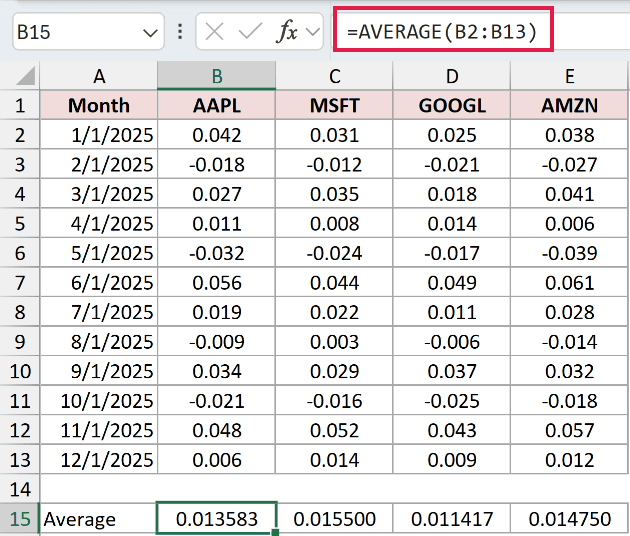
The same returns table again, this time as the starting point for the MMULT approach

The idea is to center the data first. Start by working out each stock’s average return with AVERAGE, one figure per column.

=AVERAGE(B2:B13) in cell B15 giving AAPL's mean monthly return of 0.013583, with the other three averages alongside

Then subtract each average from every value in its column. That leaves a table of deviations, how far each month sat above or below the stock’s own mean.

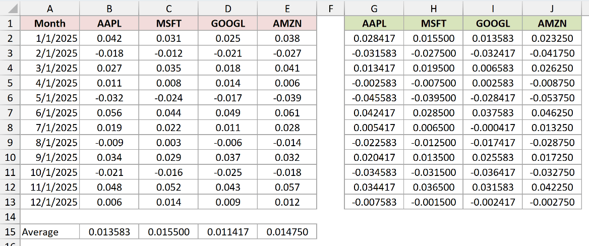
The deviation table in columns G to J, each value showing how far that month sat above or below its own stock's average

Then you multiply that deviation table by its own transpose and divide by the number of months. Here is the whole thing in one formula, entered in a single cell:

=LET(data,B2:E13,n,ROWS(data),dev,data-BYCOL(data,LAMBDA(c,AVERAGE(c))),MMULT(TRANSPOSE(dev),dev)/n)

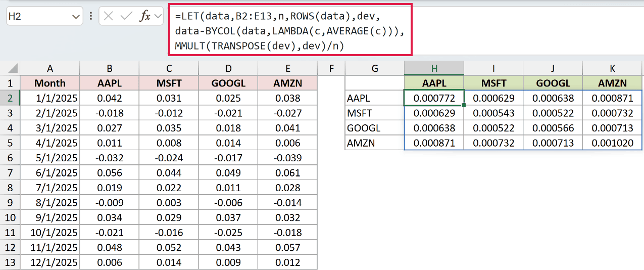
The single LET and MMULT formula in cell H2 spilling the whole four by four covariance matrix, with the four tickers as row and column labels

It spills a 4×4 matrix that matches both earlier methods. The ticker labels around it tell you which pair each figure belongs to.

How does this formula work?

BYCOL(data,LAMBDA(c,AVERAGE(c))) returns the four column averages as a single row. Subtracting that row from data centers every value on its column mean, giving the deviation table dev.

MMULT(TRANSPOSE(dev),dev) multiplies the deviations by themselves. For each pair of stocks, that sums the products of their matched deviations, which is exactly the top of the covariance formula.

Dividing by n, the number of months, finishes the population covariance. That’s why the result lines up with COVARIANCE.P and the ToolPak to the last decimal.

Note: This formula needs Excel for Microsoft 365 or Excel 2024 because BYCOL isn’t available in Excel 2021. In earlier versions, build the deviation table in cells, then use MMULT in a selected 4×4 range entered with Ctrl+Shift+Enter, dividing by the month count.

Additional Notes About the Covariance Matrix in Excel

All three methods here return population covariance, dividing by the number of rows. For a sample, use COVARIANCE.S in Method #2 or divide by one less than the count in the MMULT formula.
The diagonal of any covariance matrix is each variable’s own variance. Population variance also equals VAR.P of that column, which is a handy way to sanity-check your grid.
The ToolPak result is a snapshot. It won’t move when you change the data, so the formula methods are better whenever your returns get updated.
Keep the input columns the same length with matching numeric observations. COVARIANCE.P ignores text, logical values, and blanks, then returns #N/A if the two arrays contain different numbers of data points.
A covariance number’s size depends on the scale of the data, so it’s hard to compare across pairs. If you want a scale-free view, convert it to a correlation matrix.

Frequently Asked Questions

What’s the difference between COVARIANCE.P and COVARIANCE.S in a matrix?

COVARIANCE.P divides by the number of data points and treats them as the entire population. COVARIANCE.S divides by one less and treats them as a sample of something larger.

In a matrix, each .S value is slightly larger in magnitude, since it’s the .P value multiplied by n/(n-1). A negative covariance gets slightly more negative. The Data Analysis ToolPak always uses the population version.

How do I turn a covariance matrix into a correlation matrix?

Divide each covariance by the product of the two variables’ standard deviations. So a cell becomes cov(i,j) divided by (SDi times SDj).

You can also skip the covariance step and use CORREL on each pair, which returns the correlation directly between minus 1 and plus 1.

Do I need the Analysis ToolPak add-in enabled before I can use it?

Yes. Go to File, then Options, then Add-ins. Next to Manage Excel Add-ins, click Go, tick Analysis ToolPak, and click OK. The Data Analysis button then appears on the Data tab. This applies to Method #1 only; the formula methods work without it.

Conclusion

You now have three ways to build a covariance matrix in Excel. The Data Analysis ToolPak in Method #1 is my default when I just want the numbers fast and don’t need them to update.

If the data changes often, reach for the COVARIANCE.P grid in Method #2, or the single MMULT formula in Method #3 if you’re on Excel 365. All three land on the same matrix, so pick the one that fits how you work.

Other Excel articles you may also like: