
The IMTAN function in Excel returns the tangent of a complex number, with the answer stored as text.
A complex number has a real part and an imaginary part, written together using i or j. IMTAN keeps those parts together in its result.
I’ll show you how to use IMTAN with complex numbers, real angles, and pure imaginary inputs, then check its results and recognize input errors.
IMTAN Function Syntax in Excel
IMTAN takes a single required argument:
=IMTAN(inumber)
- inumber (required): The complex number whose tangent you want. Supply complex text using lowercase
iorj, a real number, or a cell reference containing either.
For real angles, IMTAN expects radians. The RADIANS function converts degrees to radians so IMTAN receives the angle in the units it needs.
IMTAN is available in Excel 2013 and later.
When to Use IMTAN Function
- Calculate tangents for complex numbers already stored in worksheet cells.
- Calculate a tangent when your real and imaginary input components are stored separately.
- Keep a tangent result in complex text form for further complex-number calculations.
- Check how tangents of pure imaginary inputs relate to the hyperbolic tangent.
Example 1: Calculate Tangents and Extract Their Parts
Let’s start with complex numbers already written in cells.
Below is the dataset. Column A contains complex inputs, while columns B through D have headers and empty cells for tangents and their numeric components.
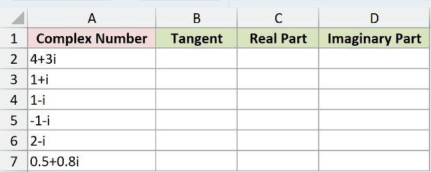
We want each tangent and its real and imaginary parts in separate columns.
Enter this formula in B2, then copy it down through B7:
=IMTAN(A2)
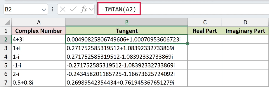
For 4+3i, the result is 0.00490825806749606+1.00070953606723i. That’s one text value, even though it contains numeric components.
A bare range passed to IMTAN returns a single #VALUE!. We’ll use individual cell references and copy each formula down throughout these examples.
IMREAL extracts the real part of IMTAN’s text result as a number. ROUND rounds that number to four decimal places for comparison.
Enter this in C2 and copy it down through C7:
=ROUND(IMREAL(B2),4)
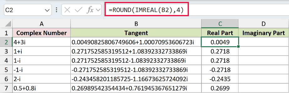
C2 displays 0.0049, the rounded real part of the tangent.
IMAGINARY extracts the imaginary coefficient as a number, without the i. Here, it lets you read and round that part of IMTAN’s result.
Enter this in D2 and copy it down through D7:
=ROUND(IMAGINARY(B2),4)
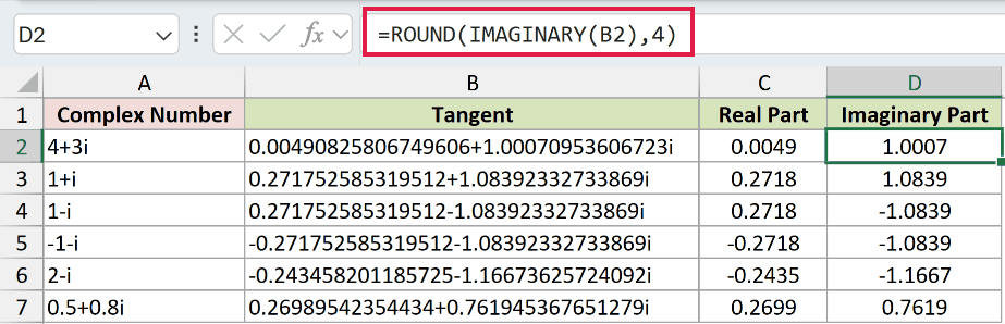
D2 displays 1.0007. You can use this extracted coefficient in ordinary numeric calculations.
Compare the 1+i and 1-i rows. Their real components both display 0.2718, while their imaginary components display 1.0839 and -1.0839.
For -1-i, both components switch sign: -0.2718 and -1.0839. The tangent changes sign when the entire input changes sign.
Pro Tip: Changing the cell’s decimal format won’t shorten an IMTAN text result. Extract its components with IMREAL and IMAGINARY, then round those numbers as shown here.
Example 2: Compare IMTAN With TAN for Degrees
TAN calculates the tangent of a real angle in radians and returns a number. Comparing it with IMTAN shows how IMTAN’s text result differs.
Below is the dataset. Column A lists angles in degrees, column B is ready for IMTAN results, and column C holds the TAN comparison scaffolding.
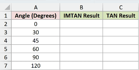
We want to compare the complex-text result with an ordinary numeric tangent after converting degrees to radians.
Enter this in B2, then copy it down through B7:
=IMTAN(RADIANS(A2))
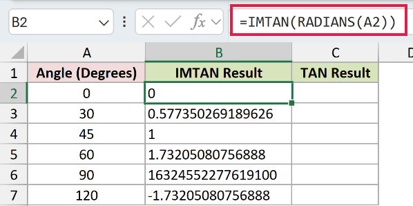
At 45 degrees, IMTAN returns the text 1. At 60 degrees, it returns 1.73205080756888.
For the TAN comparison, enter this in C2 and copy it down through C7:
=TAN(RADIANS(A2))
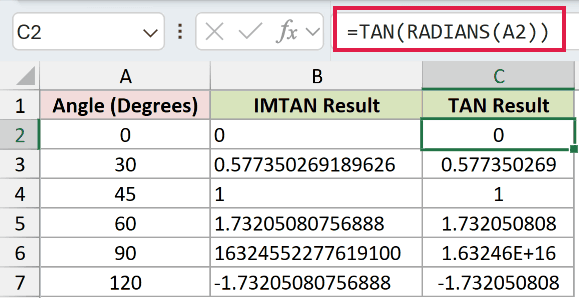
The TAN comparison displays 1 and 1.732050808 for those same angles. TAN returns numbers, while IMTAN returns text.
For ordinary real-angle calculations, I’d use TAN. IMTAN is useful when the answer needs to stay in complex text form.
At 90 degrees, IMTAN returns 16324552277619100, and the TAN comparison displays 1.63246E+16. Neither cell returns an error.
Pro Tip: Tangent is undefined at exactly 90 degrees. Excel’s finite-precision conversion produces a huge value near that point, not a valid tangent at 90 degrees.
Example 3: Calculate Tangents of Pure Imaginary Inputs
TANH calculates a number’s hyperbolic tangent. Applying it to a pure imaginary input’s coefficient gives the imaginary coefficient of IMTAN’s result.
Below is the dataset. Column A contains pure imaginary inputs, with empty result cells for IMTAN in column B and the TANH comparison in column C.
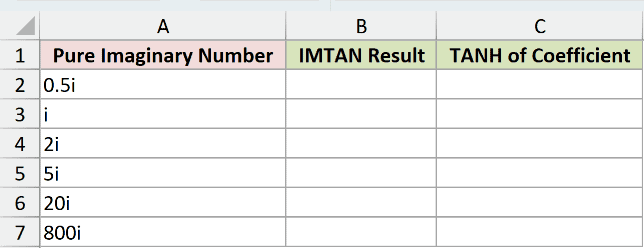
We want to calculate each imaginary tangent and compare its coefficient with the hyperbolic tangent of the input coefficient.
Enter this in B2, then copy it down through B7:
=IMTAN(A2)
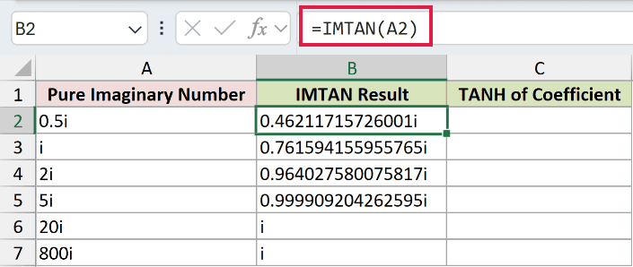
The input 0.5i returns 0.46211715726001i, while 2i returns 0.964027580075817i. Each answer remains pure imaginary.
For the TANH comparison, enter this in C2 and copy it down through C7:
=TANH(IMAGINARY(A2))
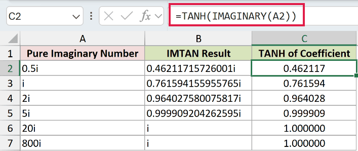
IMAGINARY extracts the input coefficient, and TANH calculates its hyperbolic tangent. The comparison displays 0.462117 for 0.5i and 0.964028 for 2i.
For a pure imaginary input, the complex tangent is the hyperbolic tangent of its coefficient, multiplied by i.
The 20i and 800i inputs both return i. Their TANH comparison cells display 1.000000; these large imaginary inputs don’t cause overflow in IMTAN.
Example 4: Build Inputs and Check the Calculation
You can also start with the real and imaginary components in separate cells.
Below is the dataset. Columns A and B hold the components; C is ready for IMTAN, while D and E contain scaffolding for a long-hand check and its difference.
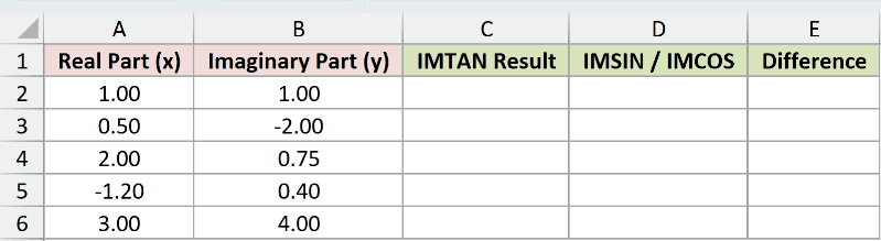
We want to build each complex input, calculate its tangent, and measure the difference from the complex sine-divided-by-cosine check.
Enter this in C2, then copy it down through C6:
=IMTAN(COMPLEX(A2,B2))
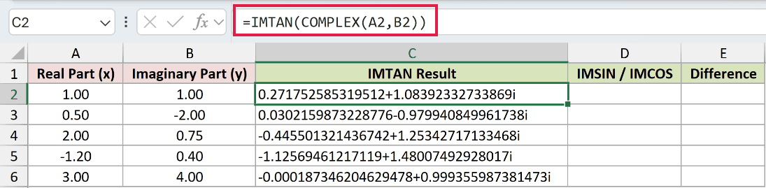
COMPLEX combines real and imaginary components into one complex number stored as text. IMTAN then calculates its tangent.
The first row returns 0.271752585319512+1.08392332733869i.
For the long-hand comparison, enter this in D2 and copy it down through D6:
=IMDIV(IMSIN(COMPLEX(A2,B2)),IMCOS(COMPLEX(A2,B2)))

IMSIN calculates the complex sine, and IMCOS calculates the complex cosine. IMDIV divides these complex values to check IMTAN using the sine-over-cosine relationship.
Its first result is 0.271752585319513+1.0839233273387i.
The final digits differ from IMTAN’s result. The methods agree to about 14 digits, but the text strings aren’t identical.
To measure that comparison difference, enter this in E2 and copy it down through E6:
=IMABS(IMSUB(C2,D2))

How this formula works:
- IMSUB subtracts the long-hand check from the IMTAN result as complex numbers.
- IMABS returns the magnitude of that difference as an ordinary number.
The comparison difference in E2 displays 1.0E-14. The last row’s comparison difference displays 6.1E-17.
Use IMTAN for the direct calculation. The longer expression is a check, and its small rounding differences don’t mean the methods calculate different mathematical functions.
Example 5: Recognize Accepted Inputs and Deliberate Errors
Let’s finish by checking which inputs IMTAN accepts.
Below is the dataset. Column A labels each input type, column B contains the test inputs, including a blank, and column C is ready for the results.
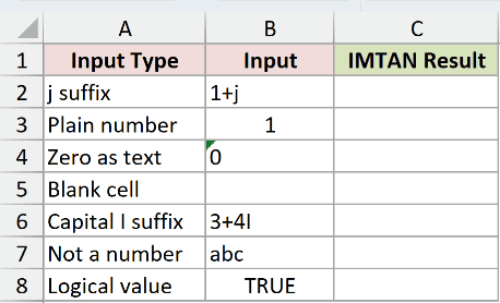
We want to see which inputs calculate successfully and why the deliberate error rows fail.
Enter this in C2, then copy it down through C8:
=IMTAN(B2)
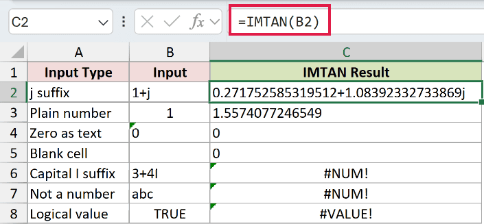
The 1+j input returns 0.271752585319512+1.08392332733869j. IMTAN accepts the lowercase j suffix and keeps it in the result.
The plain number 1 returns the text 1.5574077246549. Both the text zero and the truly blank input return the text 0.
The remaining cells deliberately show errors:
C6returns#NUM!because3+4Iuses an uppercase suffix. Change it to lowercasei.C7returns#NUM!becauseabcisn’t a valid complex number. Replace it with a numeric or complex input.C8returns#VALUE!because TRUE is a logical value. Supply the intended number instead.
A blank returning 0 can hide missing input, so check that an empty source cell really means zero before using its result.
Tips & Common Mistakes
- Keep degrees and radians straight. Convert degree inputs with RADIANS, as in the real-angle comparison. Don’t pass a degree value directly and expect a degree-based tangent.
- Unary plus enables range spilling in Excel 2021, Excel 2024 and Microsoft 365; in Excel 2019 and earlier, copy per-row formulas down.
- Treat the result as text. Extract numeric components with IMREAL and IMAGINARY, as in Example 1, before rounding or using them in ordinary numeric calculations.
- Compare numerical differences instead of text equality. Equivalent complex calculations can differ in their last digits, as the long-hand check shows.
List of All Excel Functions
