
The IMCOS function in Excel returns the cosine of a complex number as text, keeping its real and imaginary parts together in the result.
Complex numbers have a real part and an imaginary part, written with a lowercase i or j. IMCOS lets you calculate their cosine directly in a worksheet.
Changing the text output’s number format won’t shorten its decimals. You’ll need to extract the parts as numbers before formatting or calculating with them separately.
I’ll show you how to calculate complex cosines, compare real and pure imaginary inputs, and extract numeric parts for further calculations.
IMCOS Function Syntax in Excel
IMCOS takes a complex number as its required argument:
=IMCOS(inumber)
- inumber (required): The complex number whose cosine you want. Supply a cell reference, complex text in double quotes, a real number, or a value built with COMPLEX.
Complex text uses the form x+yi or x+yj, where x is the real part and y is the imaginary coefficient. Use radians for real angles.
The result is text even when no imaginary part appears. Lowercase i and j are accepted, and an input using j keeps that suffix in its complex output.
When to Use IMCOS Function
- Calculate cosines of complex values in a math worksheet.
- Compare how real and pure imaginary inputs behave.
- Obtain a complex cosine, then extract its parts for charts or numeric calculations.
- Check a complex cosine against separate trigonometric and hyperbolic calculations.
Example 1: Calculate Cosines of Complex Numbers
Let’s start with a column of complex values and look at how their signs affect the results.
Below is the dataset. Column A contains labels, column B holds complex inputs, and column C has the header and empty cells for their cosines.
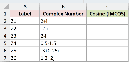
We want to calculate the cosine of each complex number in column B.
Enter this formula in C2, then copy it down to C7:
=IMCOS(B2)
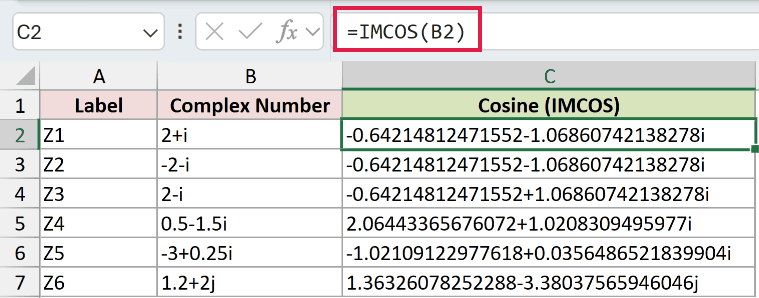
For 2+i, the result is -0.64214812471552-1.06860742138278i. The next input, -2-i, returns the identical text because reversing both signs leaves the cosine unchanged.
The input 2-i returns -0.64214812471552+1.06860742138278i. Here, only the imaginary sign changes in the input, and only the imaginary sign changes in the output.
That sign-flipped pair is called a conjugate pair.
The final input, 1.2+2j, returns 1.36326078252288-3.38037565946046j. Excel preserves the lowercase j suffix.
These formulas calculate each row separately. Passing a bare range directly to IMCOS returns a single #VALUE!, so copying down is the default method here.
Pro Tip: IMCOS can spill when its range input is first coerced into an array, such as by prefixing the range with a unary plus. That requires Excel 2021, Excel 2024, or Microsoft 365. In Excel 2019 and earlier, use the copied-down method shown here.
Example 2: Compare Real and Pure Imaginary Inputs
Some complex cosines have no imaginary part at all.
Below is the dataset. Column A holds real inputs and E holds pure imaginary inputs, with result spaces in B and F and comparison spaces in C and G.
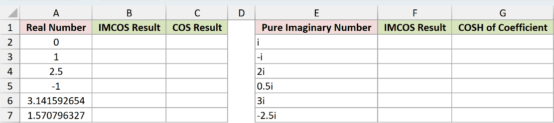
We want to compare IMCOS with COS for real inputs and COSH for pure imaginary inputs.
Enter the real-input formula in B2 and copy it down to B7:
=IMCOS(A2)
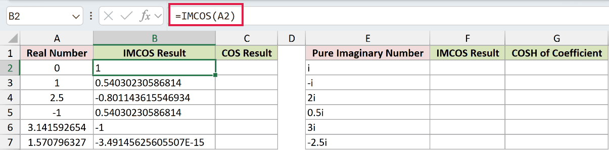
The first result is 1. For the next input, IMCOS returns 0.54030230586814. Both results are text, even though they look like ordinary numbers.
For the COS comparison, enter this in C2 and copy it down to C7:
=COS(A2)
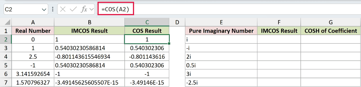
The COS comparison returns numbers. C2 displays 1, while C3 displays 0.540302306. The difference is display only, since COS returns a number shown in General format.
Near half pi, B7 shows -3.49145625605507E-15, while the COS comparison in C7 shows -3.49146E-15. These tiny floating-point residues are very close to zero.
Now enter the pure imaginary input formula in F2 and copy it down to F7:
=IMCOS(E2)
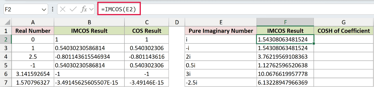
Both i and -i return 1.54308063481524. Their cosines are real-valued, although IMCOS still stores the output as text.
For the COSH comparison, enter this in G2 and copy it down to G7:
=COSH(IMAGINARY(E2))
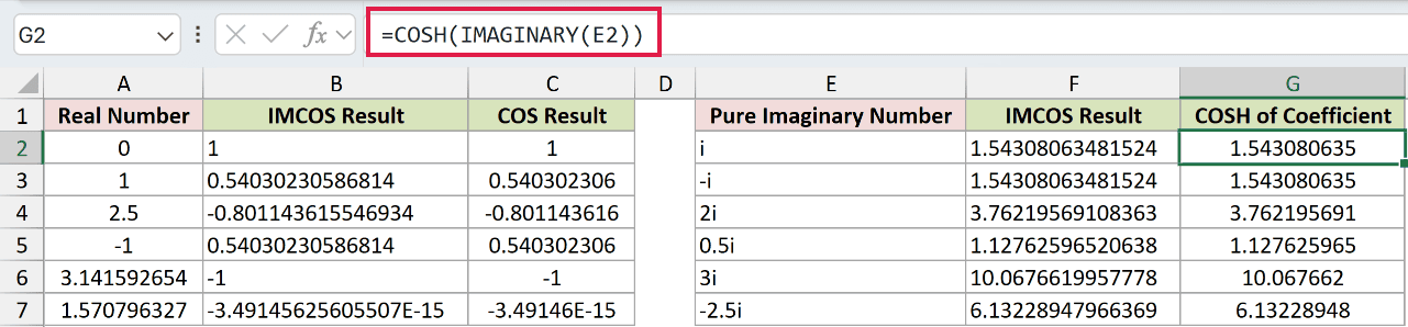
IMAGINARY extracts the imaginary coefficient, and COSH calculates its hyperbolic cosine. The comparison in G2 displays 1.543080635 as a number.
A pure imaginary input’s cosine equals the hyperbolic cosine of its coefficient. Changing the coefficient’s sign doesn’t change that result.
Use COS when your input is a real angle and you need a numeric result. The COSH comparison explains why pure imaginary inputs produce real-valued cosines.
Example 3: Extract Numeric Real and Imaginary Parts
Let’s turn the complex text output into numbers you can format or use in a chart.
Below is the dataset. Column A contains complex inputs, and columns B through D have spaces for the cosine, real part, and imaginary part.
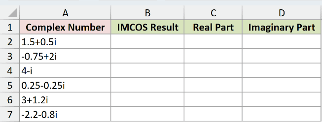
We want to calculate each cosine and separate its real and imaginary parts into numeric columns.
Start in B2, then copy down to B7:
=IMCOS(A2)
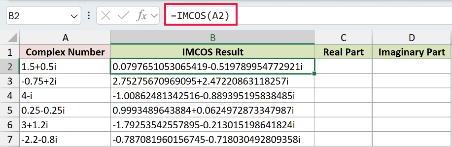
The input 1.5+0.5i returns 0.0797651053065419-0.519789954772921i. Applying a numeric format to this text won’t shorten either part.
Extract the real part in C2, then copy down to C7:
=IMREAL(B2)
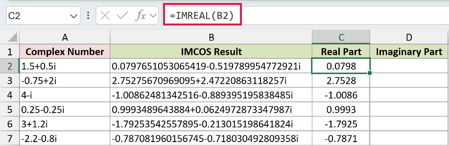
Cell C2 displays 0.0798. IMREAL returns a number, so the column’s decimal format now works.
Extract the imaginary coefficient in D2, then copy down to D7:
=IMAGINARY(B2)
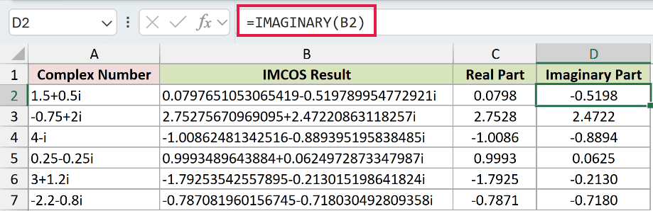
Cell D2 displays -0.5198. This is the signed coefficient without the i, ready for ordinary numeric calculations.
The next row displays 2.7528 and 2.4722 in the extracted columns. Each formula reads the cosine in column B, rather than the original input.
Pro Tip: Number formatting changes how the extracted numbers look, not their stored precision. If a later calculation needs rounded values, apply ROUND after extracting the relevant part.
Example 4: Check the Complex Cosine Calculation
Finally, let’s check the parts of the result when the input components are stored separately.
Below is the dataset. Columns A and B hold real and imaginary components. Column C has space for IMCOS; D and E will check its real and imaginary parts.
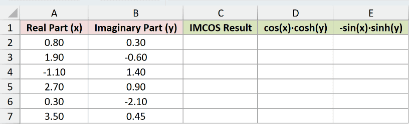
We want to build each complex input, calculate its cosine, and check the result’s components independently.
Enter this formula in C2 and copy it down to C7:
=IMCOS(COMPLEX(A2,B2))
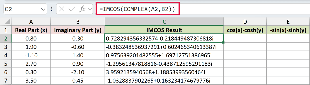
COMPLEX combines the real part in A2 with the imaginary coefficient in B2. IMCOS then calculates the cosine without needing a separate input-text column.
For the displayed inputs 0.80 and 0.30, the result is 0.728294356332574-0.218449487306818i.
To check the real component, enter this in D2 and copy it down to D7:
=COS(A2)*COSH(B2)
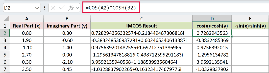
The real-component check displays 0.7282943563. It multiplies the cosine of the real input by the hyperbolic cosine of the imaginary coefficient.
To check the imaginary component, enter this in E2 and copy it down to E7:
=-SIN(A2)*SINH(B2)
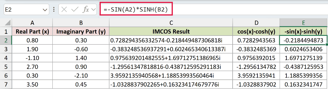
The imaginary-component check displays -0.2184494873. The leading minus sign is part of the calculation, so keep it when entering the formula.
Columns D and E only check the individual components of the complex-cosine answer in column C.
Tips & Common Mistakes
- Keep the suffix lowercase. IMCOS accepts
iorj. A capitalIreturns#NUM!, as does invalid complex text such asabc. - Don’t pass logical values. TRUE returns
#VALUE!. Supply a valid complex value or a real number instead. - Watch large imaginary parts. An input of
710ioverflows and returns#NUM!. - Treat the output as complex text. Number formatting won’t round it, and a direct SUM over complex text won’t total it. Use IMREAL or IMAGINARY to extract numeric parts, or IMABS to get the magnitude as a number.
- Round the parts before rebuilding complex text. The extract-and-rebuild method shown with IMDIV also works here. Extract each part, round it, then combine the rounded numbers with COMPLEX.
- Use radians for real angles. A degree value entered directly is interpreted as radians. Convert real angles before calculating their cosine.
- Choose the function for the input. COS is the numeric choice for real angles. IMCOS remains the function for complex cosines, with no newer replacement.
We calculated complex cosines, explored sign changes, and compared real and pure imaginary inputs with COS and COSH.
We also extracted numeric parts and checked the calculation using separate real and imaginary components.
Other Excel articles you may also like:
