
If a student has to pass every subject, you can’t just look at the average. One low score can hide behind good marks in the others.
For example, a student with 90, 85, 80, and 35 averages 72.5, but still fails a subject with a pass mark of 40.
In this article, I’ll show you how to handle the most common pass rules, from passing every subject to retests, averages, and missed exams.
Pass Only If Every Subject Is Passed
This is the most common rule. A student has to score at least the pass mark in every single subject.
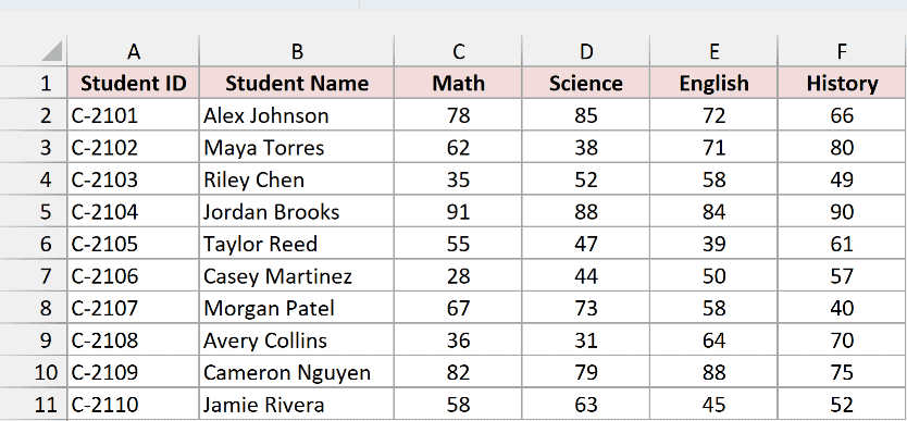
Below I have a dataset of 10 students with their marks in Math, Science, English, and History, out of 100.
The pass mark is 40 in every subject.
Here are three ways to check it.
Method #1: Using IF and AND
AND lets you write one condition per subject, so you can see exactly what’s being checked.
Enter this formula in G2 and fill it down to G11:
=IF(AND(C2>=40,D2>=40,E2>=40,F2>=40),"Pass","Fail")
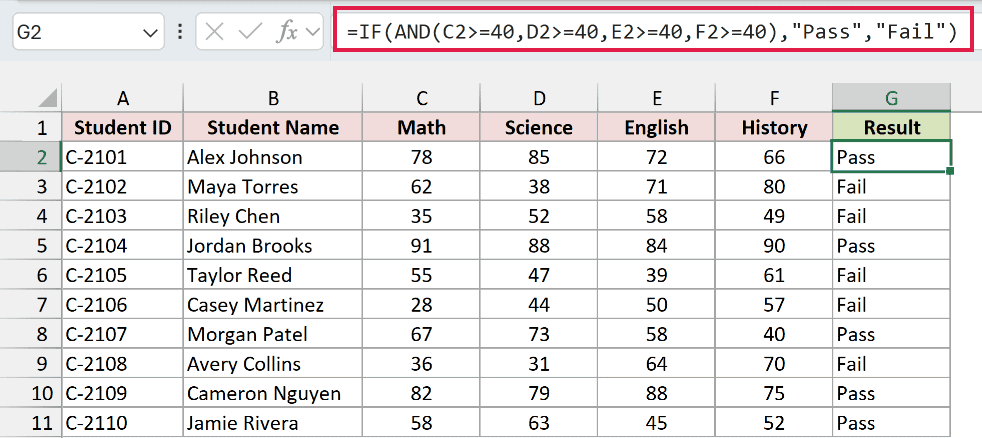
AND returns TRUE only when all four scores are 40 or more. IF then turns that TRUE or FALSE into Pass or Fail.
Maya Torres scored 38 in Science, so she fails even though her other marks are fine. Morgan Patel scored exactly 40 in History, and 40 counts as a pass.
Method #2: Using COUNTIF
Here’s another way to do this. COUNTIF counts how many subjects are below the pass mark. If that count is zero, the student passes.
Enter this formula in G2 and fill it down:
=IF(COUNTIF(C2:F2,"<40")=0,"Pass","Fail")
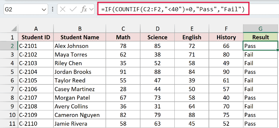
COUNTIF(C2:F2,"<40") counts the scores below 40. Avery Collins has two of them, 36 and 31, so the result is Fail.
This version is handy when you have lots of subjects, since you don’t need a separate condition for each one.
Note: COUNTIF skips blank cells, so a missing score won’t count as a fail. If your data has gaps, add the missing-score check shown later in this article.
Method #3: Using MIN
When every subject has the same pass mark, you only need to check the lowest score. If the lowest one is 40 or more, they all are.
Enter this formula in G2 and fill it down:
=IF(MIN(C2:F2)>=40,"Pass","Fail")
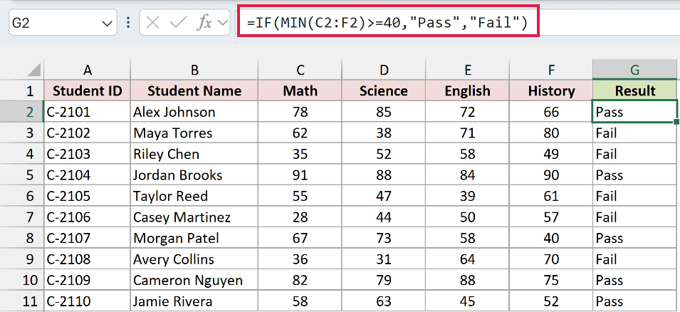
MIN returns the lowest of the four scores. For Casey Martinez, that’s 28 in Math, which is below 40, so the result is Fail.
All three methods give the same results on this data, so pick whichever formula reads best to you.
Note: Like COUNTIF, MIN ignores blank cells. A student with a missing score could show Pass, so add the missing-score check if your data isn’t complete.
Pass When Each Subject Has a Different Pass Mark
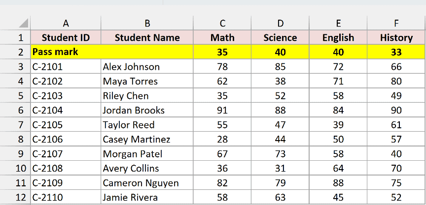
Sometimes each subject has its own pass mark. Math might need 35, while History needs only 33.
In that case, put the pass marks in their own row, right under the headers, and compare each score with the mark above it.
Below I have the same students. Row 2, highlighted in yellow, holds the pass marks: Math 35, Science 40, English 40, and History 33.
Enter this formula in G3 and fill it down to G12:
=IF(AND(C3:F3>=C$2:F$2),"Pass","Fail")
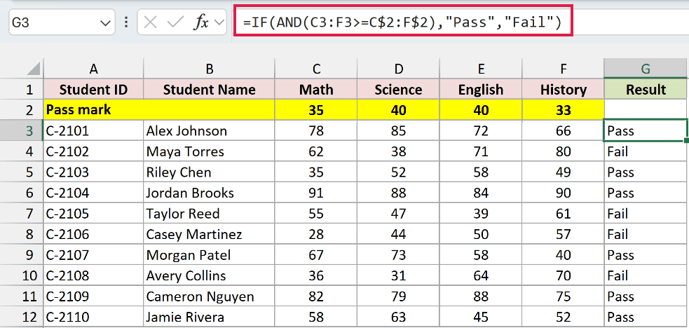
C3:F3>=C$2:F$2 compares each score with its own pass mark and returns four TRUE or FALSE values. AND returns TRUE only when all four are TRUE.
The $ before the 2 locks the pass mark row, so it stays put as you fill the formula down.
Riley Chen now passes, because the 35 in Math exactly meets the Math pass mark. Taylor Reed still fails, because 39 is below the English mark of 40.
Note: In Excel 2019 or older, confirm this formula with Ctrl + Shift + Enter, since it compares two ranges. In Microsoft 365, a regular Enter works.
Pass If a Student Clears Enough Subjects (e.g. 3 of 4)
Some schools let a student pass overall as long as they clear most subjects, even with one fail.
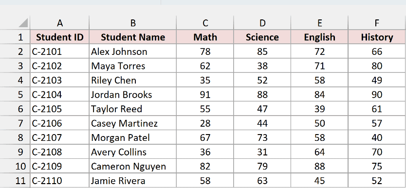
Below I have a dataset of 10 students with their marks in Math, Science, English, and History, out of 100.
A student passes with 40 or more in at least 3 of the 4 subjects.
Enter this formula in G2 and fill it down:
=IF(COUNTIF(C2:F2,">=40")>=3,"Pass","Fail")
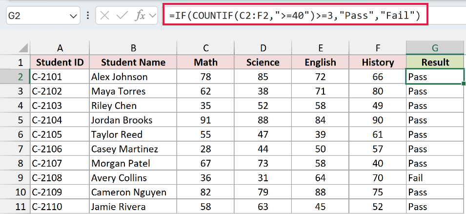
COUNTIF(C2:F2,">=40") counts how many subjects the student passed. If that count is 3 or more, the result is Pass.
Maya, Riley, Taylor, and Casey each failed one subject, but they still pass overall. Avery Collins failed two subjects, so the result is Fail.
You can also make one subject compulsory. Say Math must be passed, plus at least 3 of the 4 subjects. Use this formula in G2 instead:
=IF(AND(C2>=40,COUNTIF(C2:F2,">=40")>=3),"Pass","Fail")
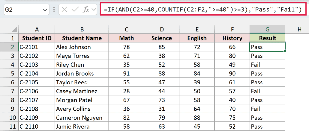
AND now needs two things: at least 40 in Math, and at least 3 passed subjects. Riley Chen and Casey Martinez now fail because of their Math scores.
Show Retest When a Student Fails Only One Subject
A lot of schools don’t fail a student over one bad subject. They give a retest instead, and only fail students who miss two or more.
Below I have a dataset of 10 students with their marks in Math, Science, English, and History, out of 100.
The pass mark is 40. One failed subject means Retest, and two or more means Fail.
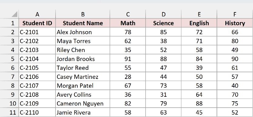
Enter this formula in G2 and fill it down:
=IF(COUNTIF(C2:F2,"<40")=0,"Pass",IF(COUNTIF(C2:F2,"<40")=1,"Retest","Fail"))
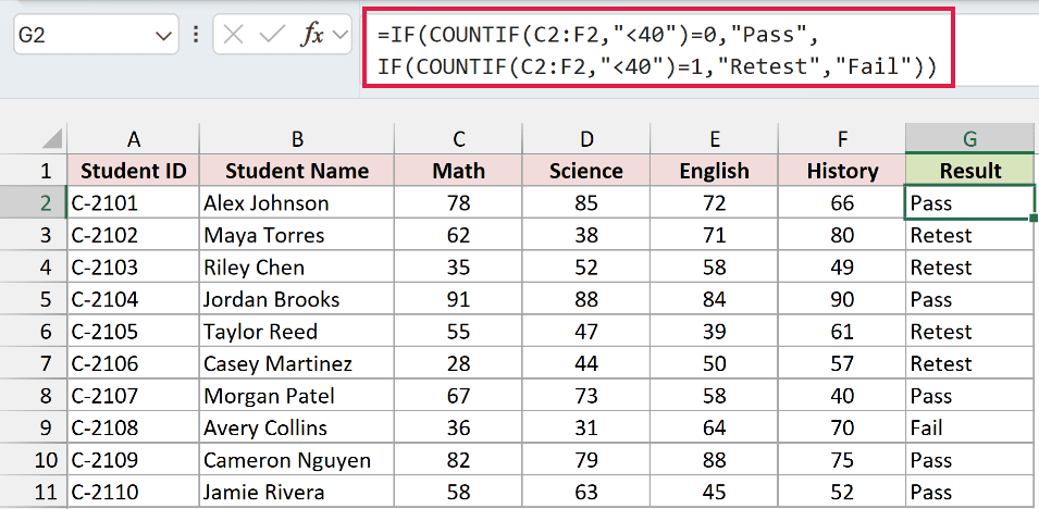
COUNTIF(C2:F2,"<40") counts the failed subjects. Zero gives Pass, exactly one gives Retest, and anything more falls through to Fail.
Maya, Riley, Taylor, and Casey each failed exactly one subject, so they get Retest. Avery Collins failed two, so the result is Fail.
Pass on Both a Minimum Score and an Overall Average
Some grading rules have two parts. The student needs a minimum score in every subject and a good overall average.
Below I have a dataset of 10 students with their marks in Math, Science, English, and History, out of 100.
Here, a student passes with at least 33 in every subject and an average of 60 or more.
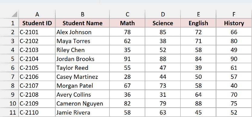
Enter this formula in G2 and fill it down:
=IF(AND(MIN(C2:F2)>=33,AVERAGE(C2:F2)>=60),"Pass","Fail")
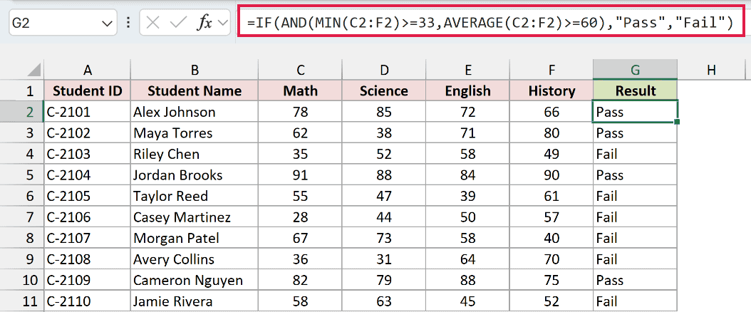
MIN checks the lowest score against 33, and AVERAGE checks the overall average against 60. AND needs both to be true.
Maya Torres passes this time, even with 38 in Science. Her lowest score clears 33, and her average is 62.75.
Morgan Patel clears every subject but misses the average, at 59.5. Avery Collins fails both parts, with 31 in Science.
Flag Students Who Missed an Exam
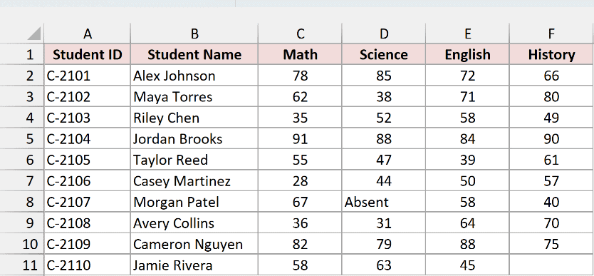
Real mark sheets often have gaps. A student misses an exam, or a teacher types Absent instead of a score.
The formulas above assume every score is there. When one is missing, some of them quietly give the wrong answer.
Below I have the same dataset with two gaps. Morgan Patel was absent for Science, and Jamie Rivera has no History score yet. The pass mark is 40.
Enter this formula in G2 and fill it down:
=IF(COUNT(C2:F2)<4,"Incomplete",IF(AND(C2>=40,D2>=40,E2>=40,F2>=40),"Pass","Fail"))
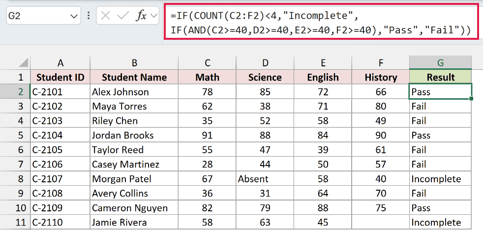
COUNT counts only the cells that hold numbers. If it finds fewer than 4, the formula returns Incomplete and skips the pass check.
Morgan and Jamie now show Incomplete, and everyone else gets their normal Pass or Fail.
Without this check, Morgan’s row would show Pass, because Excel treats the text Absent as larger than any number. Jamie’s blank would count as 0 and show Fail.
You can wrap any formula in this article the same way. Keep the COUNT part, and put your own pass rule in place of the AND part.
Count How Many Students Passed (and the Pass Rate)
Once you have a result column, counting the passes is quick. I’m using the IF and AND results from Method #1, in G2:G11.
Enter this formula in G13 to count the students who passed:
=COUNTIF(G2:G11,"Pass")
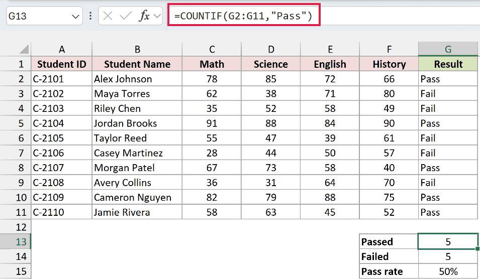
It returns 5. The same formula with “Fail” in G14 also returns 5.
To get the pass rate, divide the passes by the number of students. Enter this in G15 and format it as a percentage:
=G13/COUNTA(G2:G11)
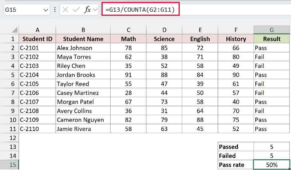
The pass rate is 50%, which is 5 out of 10 students.
Color Pass and Fail Results Automatically
A column of Pass and Fail is much easier to scan when it’s colored. Here’s how to make passes green and fails red.
Here are the steps:
- Select the results in
G2:G11.
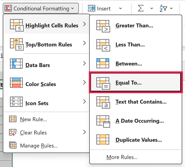
- On the Home tab, click Conditional Formatting, then Highlight Cells Rules, then Equal To.
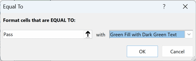
- Type Pass in the box, choose Green Fill with Dark Green Text, and click OK.
- Repeat steps 2 and 3 with Fail and Light Red Fill with Dark Red Text.
Now every Pass is green and every Fail is red.
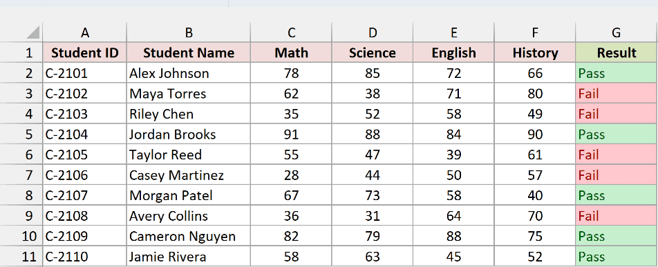
Since the rules look at the formula results, the colors update on their own whenever a score changes.
Additional Notes About Pass or Fail in Excel
- These formulas expect a number in every score cell. For blanks or text like Absent, add the COUNT check from the missed exam section.
- Change the 40 in any formula to your own pass mark. If each subject has a different mark, use a pass mark row instead.
- If you add or remove a subject, update the ranges in the formula. With the COUNT check, also change the 4 to your new number of subjects.
Frequently Asked Questions
How do I pass a student only if every subject passes?
Use the AND formula when you want to see each subject’s condition, or the MIN formula when all subjects share one pass mark.
Does a score of exactly 40 pass?
Yes. Each formula uses >=40 or counts scores <40, so a score of exactly 40 meets the requirement.
What happens when a score is blank?
It depends on the formula. AND treats a blank as 0, so the row fails. COUNTIF and MIN skip the blank, so the row can pass.
To flag it properly, use the COUNT check from the missed exam section. It returns Incomplete instead.
Can I show marks as a percentage instead of Pass or Fail?
Yes. Divide the total by the maximum marks, like =SUM(C2:F2)/400, and format the cell as a percentage. You can then use that percentage in any IF rule.
Conclusion
I showed you how to calculate pass or fail for the most common grading rules, plus how to flag missed exams and count and color the results.
If every subject has to pass, start with IF and AND. For anything more specific, pick the section that matches your school’s rule.
I hope you found this article helpful.
Other Excel articles you may also like:
