COUNTIF Function in Excel (6 Easy Examples)

If you want to count how many cells meet a certain condition, COUNTIF is the function you reach for. It checks a range and tallies up every cell that matches the rule you give it, whether that is a name, a number, or something bigger than a value.

COUNTIF gives you a single number, but in Excel 365 it also works with dynamic arrays, so you can spill a separate count for every item in a list at once. This article walks you through the syntax and six practical examples so you can start counting with confidence.

Table of Contents

COUNTIF Function Syntax in Excel

Here is how the COUNTIF function is structured:

=COUNTIF(range, criteria)

range = the cells you want to check.
criteria = the condition to match. This can be a number, text in quotes, an expression like “>200”, or a cell reference.

Text values and any comparison operators need to sit inside double quotes.

When to Use the COUNTIF Function

Counting how many times a specific name or value shows up in a list.
Finding how many numbers are above, below, or equal to a threshold.
Counting cells that contain a certain word or phrase.
Building a quick summary of how often each item appears.
Checking for duplicates by seeing if a value appears more than once.

Example 1: Count How Many Times a Name Appears

Let’s start with the most common use, counting how often a name shows up.

The dataset has two columns, Sales Rep in column A and Product in column B, across ten rows.

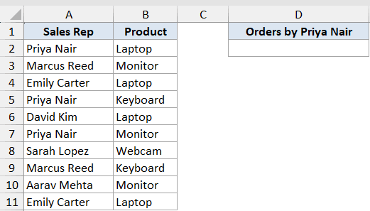
Countif Function Dataset Example 1 showing a table of sales reps and products with a header for orders by Priya Nair

We want to count how many orders were handled by Priya Nair.

Here is the formula:

=COUNTIF(A2:A11,"Priya Nair")

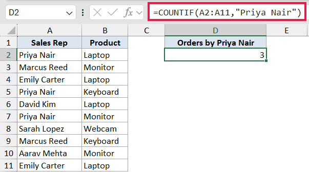
Excel formula bar showing =COUNTIF(A2:A11,"Priya Nair") with cell D2 displaying the result 3 for sales rep counts

The result is 3, since Priya Nair appears three times in column A. Notice the name is wrapped in double quotes, which is required for any text criteria.

One handy thing to know is that COUNTIF is not case-sensitive. If you typed “priya nair” instead, you would still get 3.

Example 2: Count Numbers Above a Value

Now let’s count numbers that clear a certain threshold.

This dataset has Order ID in column A and Amount in column B, across ten rows.

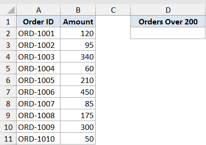
Excel dataset showing Order IDs and Amounts with a header for counting orders over 200

We want to count how many orders are over 200.

Here is the formula:

=COUNTIF(B2:B11,">200")

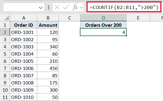
Excel formula bar showing =COUNTIF(B2:B11,">200") with the result 4 displayed in cell D2 for a list of order amounts

The result is 4, meaning four of the amounts are greater than 200. The comparison operator and the number have to be wrapped together in quotes as one string, like “>200”.

You cannot type >200 without the quotes, or Excel will throw an error. You can swap in other comparisons too, such as “<100” or “>=200”.

Example 3: Count Cells That Contain a Word

Sometimes you do not want an exact match, just cells that contain a word.

This dataset has a single column, Product Name in column A, across ten rows.

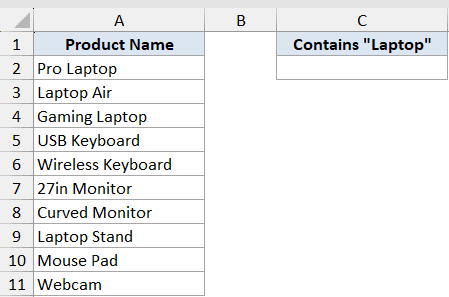
Excel dataset showing a list of products in column A and a header for counting items containing the word Laptop in cell C1

We want to count how many product names contain the word “Laptop”.

Here is the formula:

=COUNTIF(A2:A11,"*Laptop*")

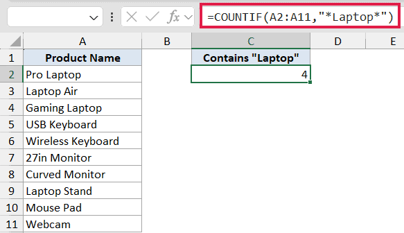
COUNTIF formula using wildcards to count cells in range A2:A11 containing the text Laptop, returning a result of 4

The result is 4, since four product names include the word Laptop somewhere in them. The asterisk (*) is a wildcard that matches any sequence of characters, so “Laptop” means “contains Laptop”.

You can change where the wildcard sits to change the match. “Laptop” finds names that begin with Laptop, “Laptop” finds names that end with it, and ? matches exactly one character.

Example 4: Count Using a Threshold From a Cell

Instead of hardcoding a number, you can pull the threshold from a cell.

This dataset has Student in column A and Score in column B, across ten rows. A Pass Mark value of 80 sits in cell D2.

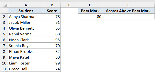
Excel dataset showing student names and scores with a pass mark of 80 to calculate scores above the threshold

We want to count how many scores are above the pass mark stored in D2.

Here is the formula:

=COUNTIF(B2:B11,">"&D2)

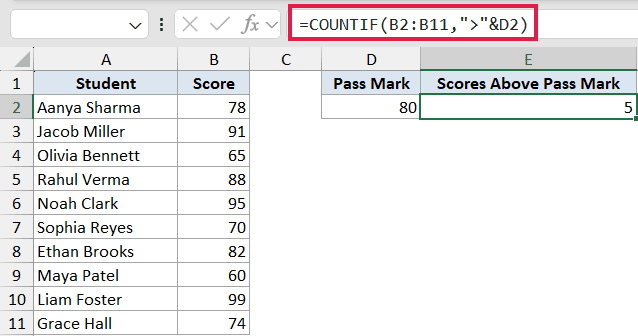
Excel formula bar showing COUNTIF(B2:B11,">"&D2) to count student scores in column B greater than pass mark 80 in cell D2

The result is 5, so five students scored above 80. To build the criteria, you join the operator (in quotes) to the cell reference using the & symbol.

The nice part is that this stays live. Change the value in D2 and the count updates on its own.

Pro Tip: The operator always stays inside the quotes and the cell reference goes outside, joined with &. Writing “>D2” inside the quotes would make Excel look for the literal text “>D2” instead of the value in the cell.

Example 5: Count Dates On or After a Date

COUNTIF handles dates just as well as numbers.

This dataset has Ticket ID in column A and Date Opened in column B, across ten rows, with dates spread through early-to-mid 2026.

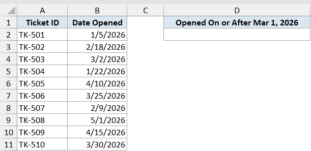
Excel dataset showing Ticket IDs and dates, with a header for counting tickets opened on or after March 1, 2026

We want to count how many tickets were opened on or after March 1, 2026.

Here is the formula:

=COUNTIF(B2:B11,">="&DATE(2026,3,1))

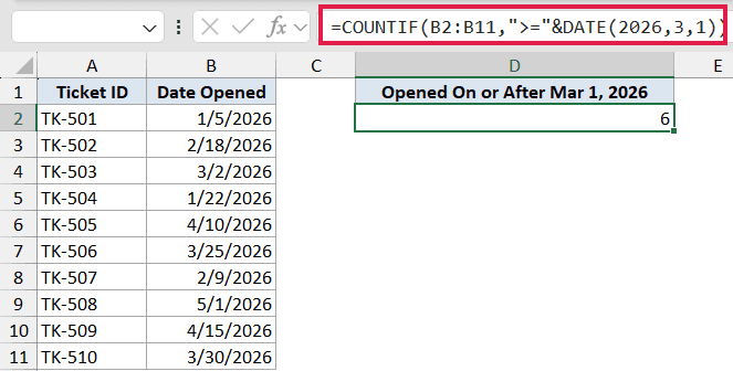
Excel formula bar showing COUNTIF with DATE function to count dates on or after March 1, 2026, returning a result of 6

The result is 6, meaning six tickets were opened on or after that date. Excel stores dates as serial numbers behind the scenes, so date comparisons work exactly like number comparisons.

Using DATE() to build the date instead of typing “3/1/2026” avoids any regional date-format problems, since DATE() is read the same way no matter your system settings.

Example 6: Count Each Unique Value at Once

This last example shows COUNTIF working with dynamic arrays.

This dataset has a single column, Department in column A, across ten rows. A small summary table sits to the right, where C2 holds =UNIQUE(A2:A11) and D2 holds the COUNTIF formula below.

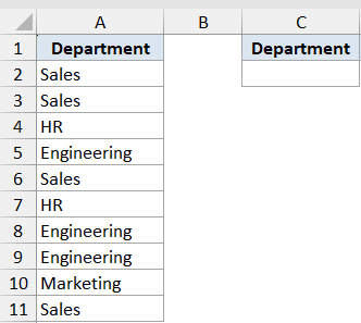
Excel dataset showing a list of departments in column A and an empty cell in column C for a COUNTIF function example

We want a count for every department in one go, without typing each name out by hand.

Here is the formula:

=COUNTIF(A2:A11,C2#)

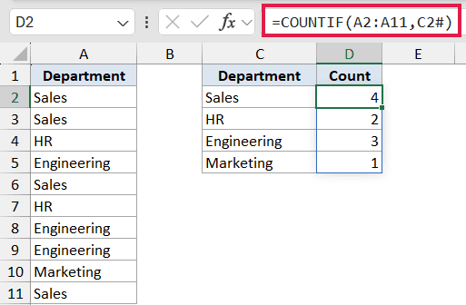
Excel formula bar showing =COUNTIF(A2:A11,C2#) to count department occurrences in a table with spills enabled

First, =UNIQUE(A2:A11) in C2 spills the list of distinct departments down the column. Then COUNTIF is fed that spilled list using the # (spill) reference C2#, which points at the whole spilled range.

The result is one count per department spilling down automatically, here 4, 2, 3, and 1. This replaces the old chore of copying a COUNTIF formula down a column row by row.

Tips and Common Mistakes

COUNTIF is not case-sensitive, so “apple” and “APPLE” count as the same. If you need case-sensitivity, use SUMPRODUCT together with EXACT.
For more than one condition at a time, use COUNTIFS instead of trying to stack COUNTIF.
If you just want to count cells with numbers, use COUNT, and for all non-empty cells use COUNTA.
Always wrap text and comparison operators in double quotes, and join cell references with the & symbol.
COUNTIF can return wrong results when matching text strings longer than 255 characters, so watch out with very long values.

That covers the main ways to count with COUNTIF, from a plain name match to numbers, wildcards, cell-based thresholds, and dates. The spilled UNIQUE version is the one most people have not tried yet, so keep it in mind when you need a quick breakdown by category. Pick the example closest to your data and tweak it from there.

List of All Excel Functions

Related Excel Functions / Articles: