
Excel’s ACOSH function returns the inverse hyperbolic cosine of a real number equal to or greater than 1.
When a value came from COSH, ACOSH recovers its nonnegative input. COSH treats positive and negative inputs alike, so ACOSH cannot recover the original sign.
In this article, I’ll show you how to calculate ACOSH for a range, reverse COSH results, validate imported values, and audit the calculation.
ACOSH Function Syntax in Excel
The ACOSH function has one required argument:
=ACOSH(number)
numberis a real number equal to or greater than 1.
When to Use ACOSH Function
- Reverse a value produced by the COSH function
- Process a list of valid hyperbolic cosine values
- Validate imported ratios before calculating their inverse hyperbolic cosine
- Check a model against the equivalent logarithmic expression
Example 1: Calculate ACOSH for a Range
Let’s start with a range of valid values.
The dataset has test IDs in column A, valid inputs in column B, and an empty result column for the inverse hyperbolic cosine.
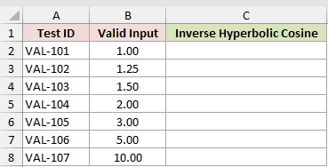
I want one ACOSH result for every value in B2:B8.
Here is the formula:
=ACOSH(B2:B8)
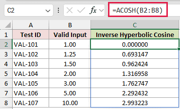
The formula starts at C2 and spills through C8. An input of 1 returns 0, while an input of 10 returns approximately 2.993223.
In Excel 2021, Excel 2024, Microsoft 365, and Excel for the web, entering the formula once fills the result range automatically.
Pro Tip: Keep the cells below C2 empty. Any value blocking the intended output range causes a #SPILL! error.
Example 2: Reverse COSH Results
This example shows what ACOSH can and cannot recover.
The dataset lists signed parameters in column B. Columns C and D hold the COSH output and the recovered ACOSH result.
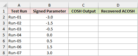
I want to calculate COSH first, then reverse those values with ACOSH.
Here is the COSH formula:
=COSH(B2:B8)
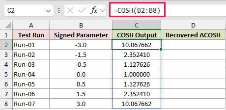
COSH returns the same value for positive and negative inputs of equal size. For example, both -3 and 3 return approximately 10.067662.
Now recover the parameter magnitude with ACOSH:
=ACOSH(C2:C8)
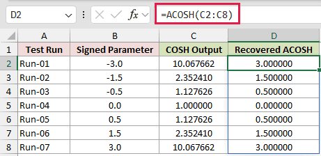
The recovered results in column D are all nonnegative. ACOSH returns 3 for both original inputs, -3 and 3.
That happens because COSH is an even function. Once COSH removes the sign, ACOSH has no information from which to restore it.
Example 3: Validate Inputs Before ACOSH
Imported data often includes values outside the ACOSH domain.
The dataset has import IDs in column A, incoming ratios in column B, and an empty checked-result column in C.
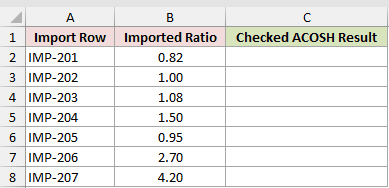
I want valid ratios calculated and values below 1 flagged for review.
Here is the formula:
=IF(B2:B8>=1,ACOSH(B2:B8),"Check source value")
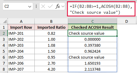
IF checks each imported ratio before ACOSH runs. Values of 1 or more return a number, while lower values return the message “Check source value.”
Without that check, an input below 1 returns the #NUM! error because no real ACOSH result exists for it.
Pro Tip: Use a clear review message instead of hiding invalid data with IFERROR. That makes a bad source value easier to find and correct.
Example 4: Audit the ACOSH Calculation
You may want a transparent check for a technical model.
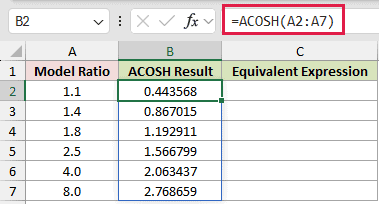
The dataset lists model ratios in column A. Columns B and C hold the ACOSH result and its equivalent logarithmic calculation.
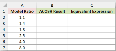
I want to compare Excel’s built-in result with the mathematical expression for the same valid inputs.
First, calculate the built-in ACOSH results:
=ACOSH(A2:A7)
Now calculate the equivalent expression:
=LN(A2:A7+SQRT(A2:A7^2-1))
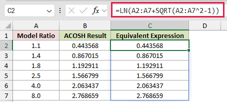
The two result columns match across the six inputs. For 1.1, both formulas return approximately 0.443568.
The built-in ACOSH formula is easier to read. The logarithmic version is useful when you need to show how an audit value was calculated.
Tips & Common Mistakes
- ACOSH accepts only real numbers equal to or greater than 1. A smaller number returns
#NUM!. - ACOSH returns a hyperbolic value. Do not treat it as a circular angle or convert it with DEGREES.
- Range formulas spill in Excel 2021, Excel 2024, Microsoft 365, and Excel for the web. Excel 2019 and earlier need per-row formulas or legacy array entry.
- Edit a spilling formula from its top-left cell. The other cells in the spill range display results but do not hold separate formulas.
- There is no newer replacement for ACOSH. The built-in function remains the clearest choice for valid inputs.
I covered range calculations, COSH reversal, input checks, and an equivalent expression for auditing ACOSH results.
I hope you found this article helpful.
Other Excel articles you may also like:
