
Excel’s ATANH function returns the inverse hyperbolic tangent of a number between minus 1 and 1.
For a correlation coefficient, this result is the Fisher z-transformation. It stretches values near either limit, which helps with statistical comparisons and intervals.
In this article, I’ll show you how to transform correlations, average them correctly, and build a confidence interval.
ATANH Function Syntax in Excel
The ATANH function has one required argument.
=ATANH(number)
- number (required) is a real number strictly between minus 1 and 1.
When to Use ATANH Function
- Convert correlation coefficients to Fisher z values before statistical analysis.
- Average several correlations without averaging the raw coefficients directly.
- Calculate confidence limits for a correlation coefficient.
- Compare correlations from two independent samples.
- Estimate the sample size needed to detect a target correlation.
Example 1: Convert Correlations to Fisher Z
Let’s start with survey questions and their correlations with overall satisfaction.
Below is the dataset. Columns A and B contain the questions and correlations. The green Fisher z header and empty cells in column C show where results will appear.
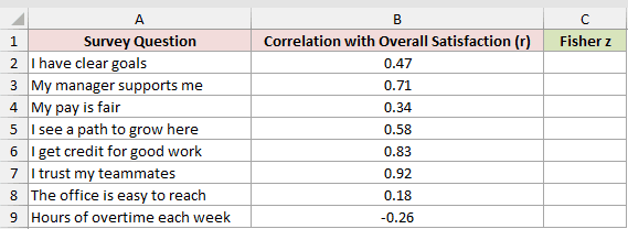
The formula will fill column C with the Fisher z value for every correlation.
Here is the formula entered in C2:
=ATANH(B2:B9)
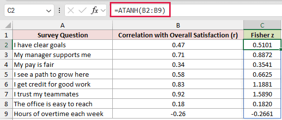
One formula returns all eight results. The correlation 0.47 becomes 0.5101, while 0.92 becomes 1.5890.
The transformation keeps the sign. The negative correlation of -0.26 returns -0.2661.
Range input spills in Excel 2021, Excel 2024, and Microsoft 365. In Excel 2019 and earlier, enter =ATANH(B2) and fill it down.
Pro Tip: Keep C2:C9 clear before entering the formula. Any occupied cell in the output area can cause a #SPILL! error.
Example 2: Compare ATANH, FISHER, and LN
Now let’s verify the calculation in three different ways and then reverse it.
Below is the dataset. Column A contains correlations. Four green result columns have empty cells for ATANH, FISHER, the expanded LN calculation, and the inverse result.
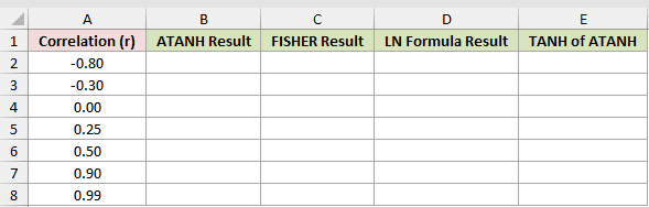
First, we’ll use ATANH to transform every correlation in column B.
Here is the formula entered in B2:
=ATANH(A2:A8)
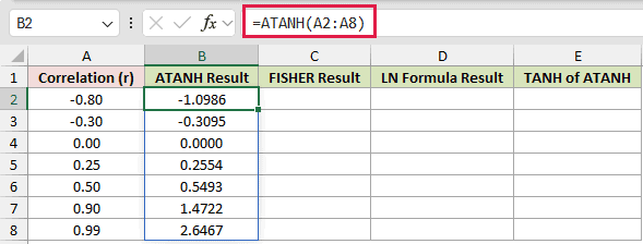
Next, FISHER calculates the same z values in column C.
Here is the formula entered in C2:
=FISHER(A2:A8)
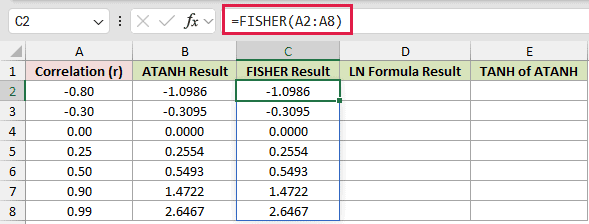
Column D rebuilds the transformation from its logarithmic definition.
Here is the formula entered in D2:
=0.5*LN((1+A2:A8)/(1-A2:A8))
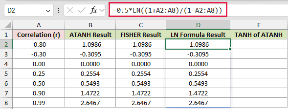
Finally, TANH converts the ATANH results back to their original correlations in column E.
Here is the formula entered in E2:
=TANH(B2:B8)
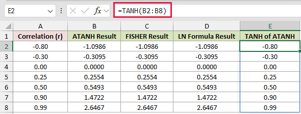
Columns B, C, and D match at every displayed value. For example, all three methods return 0.5493 when the correlation is 0.50.
TANH reverses ATANH, so column E reproduces the correlations in column A. FISHERINV can perform the same statistical inverse operation.
Notice how quickly z grows near 1. A correlation of 0.90 returns 1.4722. At 0.99, the result is 2.6467.
Example 3: Average Several Correlations Correctly
Here’s a store comparison where each correlation comes from a different number of tracked days.
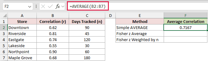
Below is the dataset. Columns A:C list each store, the correlation between daily foot traffic and daily sales, and the number of days tracked.
The E:F card includes the Method and green Average Correlation headers, plus labeled empty cells for Simple AVERAGE, Fisher z Average, and Fisher z Weighted by n.
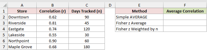
We’ll compare a plain average with two averages that use Fisher z values.
Here is the simple average formula in F2:
=AVERAGE(B2:B7)
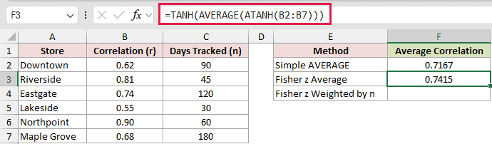
Next, F3 should transform the correlations, average the z values, and convert the result back to r.
Here is the formula:
=TANH(AVERAGE(ATANH(B2:B7)))
In Excel 2019 and earlier, confirm this formula with Ctrl+Shift+Enter.
The final method should also weight each transformed value by its sample size minus 3.
Here is the formula in F4:
=TANH(SUMPRODUCT(ATANH(B2:B7),C2:C7-3)/SUM(C2:C7-3))
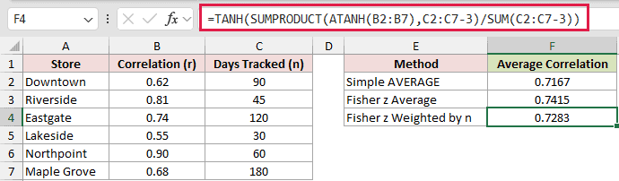
The plain average is 0.7167. Averaging in Fisher z space returns 0.7415, so the raw average runs low for these strong correlations.
The weighted method returns 0.7283. Stores tracked for more days contribute more because their n-3 weights are larger.
Example 4: Calculate a Correlation Confidence Interval
Let’s build a 95% confidence interval for one correlation, one step at a time.
Below is the dataset. The card contains r, sample size, and confidence level.
Five labeled, empty cells will hold Fisher z, two supporting values (standard error and critical z), and the lower and upper limits.
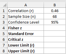
We want the limits for the 0.46 correlation between loyalty emails opened and repeat purchases for 68 customers.
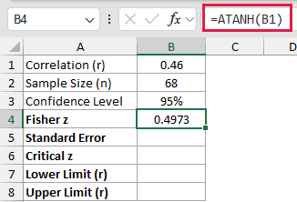
First, B4 transforms the correlation to Fisher z.
=ATANH(B1)
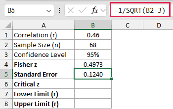
Next, B5 calculates the standard error in z space.
=1/SQRT(B2-3)
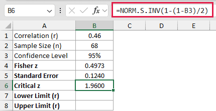
B6 converts the 95% confidence level into its critical z value.
=NORM.S.INV(1-(1-B3)/2)
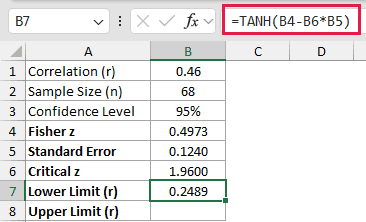
B7 subtracts the margin in z space and uses TANH to return to correlation units.
=TANH(B4-B6*B5)
B8 adds the margin and converts the upper endpoint back to r.
=TANH(B4+B6*B5)
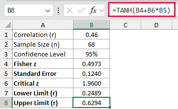
The intermediate values are 0.4973 for Fisher z, 0.1240 for standard error, and 1.9600 for the critical z value.
The resulting interval runs from 0.2489 to 0.6294. It is asymmetric around 0.46 because the calculation returns from z space to the bounded correlation scale.
Example 5: Compare Two Independent Correlations
Now let’s test whether online and in-store correlations differ across five metric pairs.
Below is the dataset. Column A holds the metric pair names, while B:E hold the online and in-store r and n values.
The green z statistic and p-value columns contain empty cells for the test results.
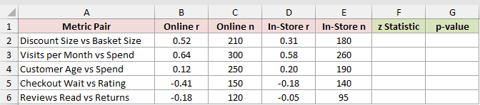
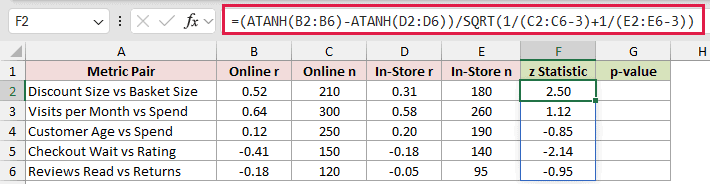
The first calculation measures each transformed difference in column F.
Here is the formula entered in F2:
=(ATANH(B2:B6)-ATANH(D2:D6))/SQRT(1/(C2:C6-3)+1/(E2:E6-3))
We then turn each z statistic into a two-tailed p-value in column G.
Here is the formula entered in G2:
=2*(1-NORM.S.DIST(ABS(F2:F6),TRUE))
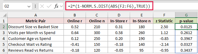
The first metric pair returns a p-value of 0.0125. Checkout wait versus rating returns 0.0327.
Both fall below 0.05. The other three p-values stay above that threshold in this dataset.
Pro Tip: This test assumes the two correlations come from independent samples, such as different online and in-store customers. It does not cover two correlations measured on the same people.
Example 6: Estimate Sample Size for Correlation
Here’s a planning table for several target correlation strengths.
Below is the dataset. Column A lists target correlations. Column B has a green header and empty results, while D:E contains the 5% significance and 80% power settings.
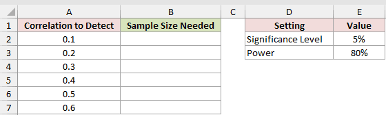
The formula returns the required sample size for each target correlation in column B.
Here is the formula entered in B2:
=ROUNDUP(((NORM.S.INV(1-$E$2/2)+NORM.S.INV($E$3))/ATANH(A2:A7))^2+3,0)
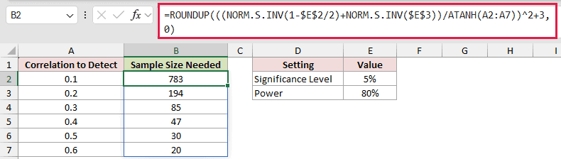
The formula finds the critical values for significance and power, divides their sum by the Fisher z value, squares the result, and adds 3.
For r 0.1, the unrounded result is 782.65. ROUNDUP takes it to the next whole observation, 783, so the planned sample never falls short of the target.
By comparison, r 0.6 requires 20 observations with the same settings.
Weak correlations need much larger samples to detect under the same significance and power targets.
Example 7: Handle Invalid ATANH Inputs
The last example shows valid inputs, boundary values, a blank cell, and text.
Below is the dataset. Columns A and B identify each scenario and input. The green result column has empty cells for values or errors returned by ATANH.
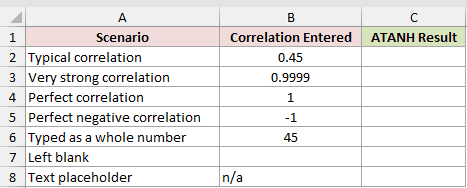
The results in column C will show how ATANH handles each listed input.
Here is the formula entered in C2:
=ATANH(B2:B8)
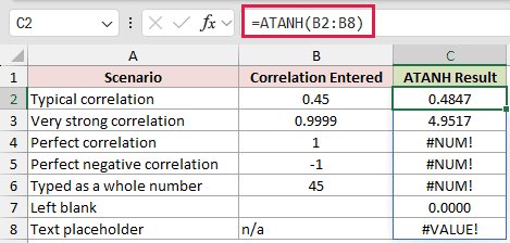
The valid inputs 0.45 and 0.9999 return 0.4847 and 4.9517. Values of 1, -1, and 45 return #NUM!.
ATANH accepts only values strictly between minus 1 and 1. A percentage entered as 45 instead of 45% is therefore outside the allowed range.
A blank cell returns 0.0000, which can look like a genuine zero correlation. The text placeholder n/a returns #VALUE!.
Pro Tip: If a perfect correlation came from CORREL, check whether the two source columns are identical or copied from each other.
Tips & Common Mistakes
- Keep the input strictly between minus 1 and 1. Either boundary returns
#NUM!. - A typed TRUE value is treated as 1 and returns
#NUM!. Numeric text such as"0.5"is converted and returns a number. - Do not treat blanks as missing automatically. A blank cell returns zero, so check the source data before interpreting the result.
- If an occupied cell blocks a spilled range, Excel returns
#SPILL!. Clear the output area or use a single-cell formula and fill down. - An implicit-intersection formula such as
@ATANH(B2:B9)collapses the range to one result. Remove the@when you intend to spill.
ATANH turns bounded correlations into Fisher z values that are easier to average, compare, and use in interval calculations.
TANH brings those results back to the original correlation scale when the analysis is complete.
Related Excel Functions / Articles:
