
The DSTDEV function in Excel estimates the sample standard deviation of values from database records that meet specified criteria.
It’s useful when your worksheet is arranged as a list with headers and you want to measure how much a filtered sample varies.
I’ll show you how to compare carriers, analyze an August shipping window, and guard against a one-match #DIV/0! error.
DSTDEV Function Syntax in Excel
The DSTDEV function uses a database, a field to measure, and a criteria range.
=DSTDEV(database, field, criteria)
- database is the full list, including its header row.
- field is the column to measure. Enter its header in quotation marks or use its position in the database.
- criteria is a separate range containing matching database headers and the conditions below them.
When to Use DSTDEV Function
- Measure variation in a sample selected from a larger list.
- Compare consistency across carriers, depots, routes, or other groups.
- Apply multiple conditions using AND or OR criteria.
- Filter records by dates, comparison operators, or wildcard text.
- Calculate sample standard deviation without manually extracting matching rows.
Example 1: Calculate Standard Deviation by Carrier
Let’s start with one text criterion.
Below is the shipment dataset with carrier and transit-hour inputs, a carrier criteria block, and an empty result cell for the sample standard deviation.
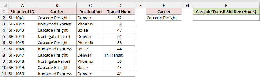
We want to measure the variation in transit hours for Cascade Freight shipments.
Here is the formula:
=DSTDEV(A1:D11,"Transit Hours",F1:F2)
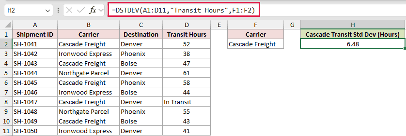
The database is A1:D11, the measured field is Transit Hours, and F1:F2 identifies the carrier to include.
DSTDEV returns 6.48 hours. The Transit Hours entry for shipment SH-1047 is text, so DSTDEV skips it.
The result uses the four numeric Cascade Freight times: 52, 47, 58, and 43.
Example 2: Use Multiple AND Criteria
Now let’s narrow the records with two conditions.
Below is the delivery dataset with Depot, Service Level, and Delivery Minutes inputs, an Eastside and Same Day criteria row, and an empty standard-deviation result cell.
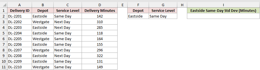
We want the sample standard deviation for Eastside deliveries using the Same Day service level.
Here is the formula:
=DSTDEV(A1:D11,4,F1:G2)
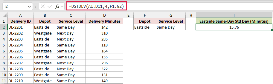
Because Eastside and Same Day sit on the same criteria row, a record must meet both conditions. The result is 15.76 minutes.
The 4 selects the fourth database column, Delivery Minutes. A quoted header is usually safer if someone may insert or move columns later.
Example 3: Compare Carrier Delivery Consistency
Here’s where the standard deviation becomes useful for a decision.
Below is the load dataset with carrier and transit-day inputs, two carrier criteria blocks, and separate result cells for comparing their sample standard deviations.
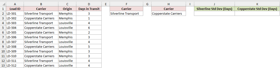
We want to compare how consistently Silverline Transport and Copperstate Carriers deliver their loads.
Here is the Silverline formula:
=DSTDEV(A1:D13,"Days in Transit",F1:F2)
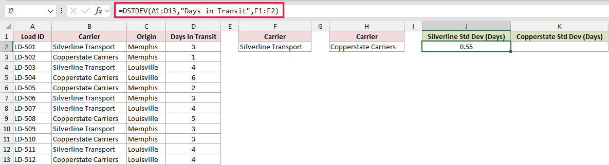
And here is the Copperstate formula:
=DSTDEV(A1:D13,"Days in Transit",H1:H2)
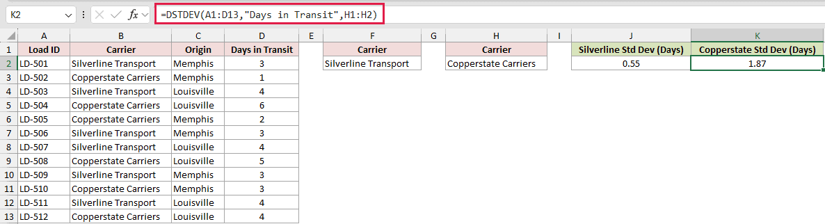
Both carriers average exactly 3.5 days, but their delivery patterns differ. Silverline returns 0.55 days, while Copperstate returns 1.87 days.
Silverline’s lower standard deviation means its delivery times are more predictable, even though the two carriers have the same average.
Example 4: Apply OR Criteria Across Warehouses
You can also combine records from more than one group.
Below is the appointment dataset with warehouse and unload-time inputs, a Warehouse criteria header, two condition rows for Reno and Sacramento, and an empty pooled-sample result cell.
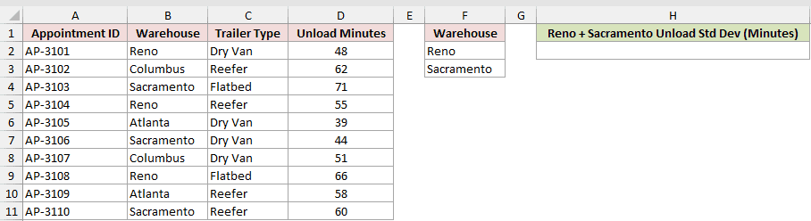
We want one sample standard deviation for appointments at either Reno or Sacramento.
Here is the formula:
=DSTDEV(A1:D11,"Unload Minutes",F1:F3)
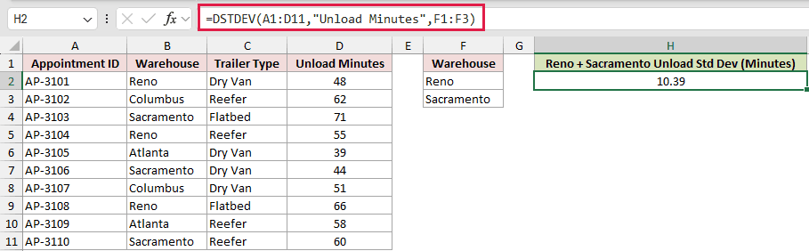
Reno and Sacramento appear on separate rows under the same header, so Excel treats them as OR conditions.
DSTDEV pools the matching unload times into one sample and returns 10.39 minutes.
Example 5: Use a Date Range With DSTDEV
Date criteria work well for period-based reviews.
Below is the order dataset with ship dates and pick-to-ship hours, two Ship Date criteria columns, and an empty result cell for the August sample.
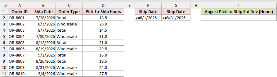
We want the sample standard deviation of pick-to-ship hours for orders shipped during August.
Here is the formula:
=DSTDEV(A1:D11,"Pick-to-Ship Hours",F1:G2)
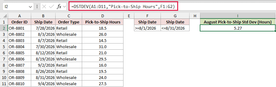
Both conditions sit on one criteria row under two Ship Date headers, so a record must pass both conditions.
The entries are >=8/1/2026 in F2 and <=8/31/2026 in G2.
The ending condition is inclusive, so the August 31 order is counted. DSTDEV returns 5.27 hours.
Example 6: Match Destinations With a Wildcard
A wildcard can match text found within a destination.
Below is the order dataset with customer, destination, and transit-hour inputs, a destination wildcard criterion, and an empty result cell for Texas orders.
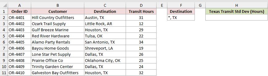
We want the sample standard deviation for orders whose destination contains “, TX”.
Here is the formula:
=DSTDEV(A1:D11,"Transit Hours",F1:F2)
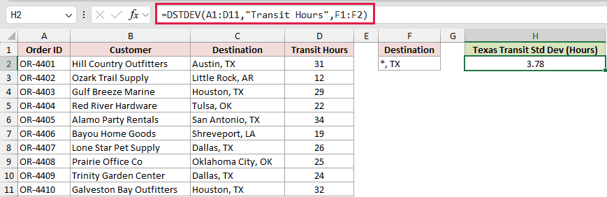
The criterion *, TX matches destinations containing “, TX”. The * covers the city in front, and Excel’s implied trailing wildcard covers anything after.
The six matching Texas orders return a sample standard deviation of 3.78 hours.
For a strict ends-with match, use ="=*, TX" in the criteria cell.
Example 7: Avoid #DIV/0! for One Match
DSTDEV needs enough matching values to estimate a sample standard deviation.
Below is the pickup dataset with carrier and late-minute inputs, one carrier criterion, and cells for the unguarded result and a checked result.
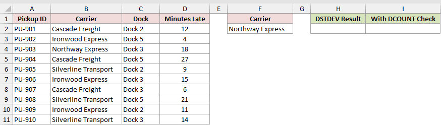
We first want to see what happens when the criteria match only one pickup.
Here is the unguarded formula that demonstrates the problem:
=DSTDEV(A1:D11,"Minutes Late",F1:F2)
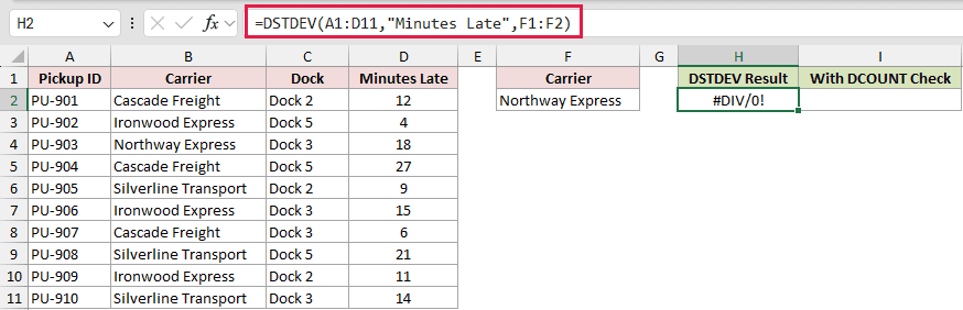
The formula deliberately returns #DIV/0! because Northway Express has only one matching numeric pickup. One value is not enough for a sample standard deviation.
Here is the guarded formula:
=IF(DCOUNT(A1:D11,"Minutes Late",F1:F2)<2,"Need 2+ pickups",DSTDEV(A1:D11,"Minutes Late",F1:F2))
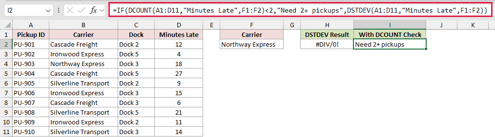
DCOUNT checks how many numeric records meet the criteria before DSTDEV runs. The guarded cell returns “Need 2+ pickups” instead of the error.
Pro Tip: Don’t hide this case with IFERROR. Checking the count tells whoever uses the worksheet what’s wrong and prevents unrelated errors from being masked.
Example 8: Compare DSTDEV With STDEV.S and FILTER
You can produce the same statistic without a database criteria block.
Below is the route dataset with driver and minutes-per-stop inputs, one driver criterion, and result cells for DSTDEV and STDEV.S with FILTER.
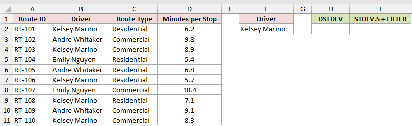
We want to compare the database-function result with a modern filtered-array formula for Kelsey Marino.
Here is the DSTDEV formula:
=DSTDEV(A1:D11,"Minutes per Stop",F1:F2)
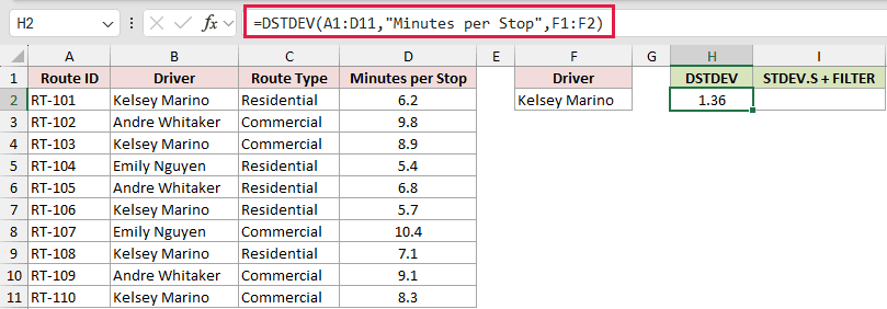
And here is the STDEV.S with FILTER comparison:
=STDEV.S(FILTER(D2:D11,B2:B11=F2))
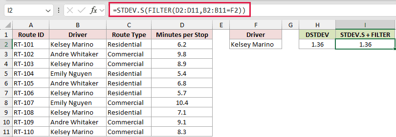
Both formulas return 1.36 minutes. DSTDEV uses the separate criteria range, while FILTER passes Kelsey Marino’s matching values directly to STDEV.S.
FILTER uses an exact comparison here. DSTDEV’s plain text criterion matches from the start of a cell, so the two approaches can differ when names share prefixes.
FILTER requires Excel 2021 or later. DSTDEV works in every current version of Excel.
Tips & Common Mistakes
- Use DSTDEV when the matching records are a sample of a larger process. Use DSTDEVP when they are the complete population you want to describe.
- With exactly one numeric match, DSTDEV returns
#DIV/0!, while DSTDEVP returns 0. With no matches, both return#DIV/0!. - Keep the criteria block beside the database, not below it. New database rows could otherwise grow into the criteria area.
- Conditions on the same criteria row use AND logic. Conditions on separate rows use OR logic.
- Plain text criteria match from the beginning. Use an exact criterion such as
="=Mall"when “Mall” must not also match “Mall Kiosk”. - To avoid depending on typed date text, build the criteria with
=">="&DATE(2026,8,1)and="<="&DATE(2026,8,31). The result is the same. - A misspelled field name returns
#VALUE!. A misspelled criteria header can leave no matching records and cause#DIV/0!. - DSTDEV skips text in the measured field. Make sure text entries are intentional before trusting the result.
- Excel has no STDEVIFS function. In Excel 2021 and later, STDEV.S with FILTER is the more flexible route for calculated conditions or one result per group.
DSTDEV works best when your list already uses database-style headers and the selected records represent a sample.
The most important check is the match count. Fewer than two numeric records can’t produce a sample standard deviation.
Related Excel Functions / Articles:
