
The GESTEP function in Excel returns 1 when a number is greater than or equal to a threshold, and 0 when it falls below it.
Those results work as numeric flags. You can add them to count days a goal was met, or multiply them by an incentive amount to calculate payouts.
Equality matters here. Reaching a target exactly counts as passing it, so GESTEP suits rules written as “at least” rather than “more than.”
I’ll show you how to flag targets, build loyalty tiers, and fix the range-input error that can stop a GESTEP count from working.
GESTEP Function Syntax in Excel
GESTEP compares a number with an optional threshold called step:
=GESTEP(number, [step])
- number (required): The number you want to test, or a cell containing it.
- step (optional): The threshold to compare against. If you leave it out, GESTEP uses 0.
The result is a number, not TRUE or FALSE. A value equal to step returns 1; a value below it returns 0.
When to Use GESTEP Function
- Flag entries that meet a fixed goal, then add the flags to count qualifying entries.
- Compare each store’s performance with its own target and calculate an incentive.
- Identify changes that are nonnegative, including periods with no change.
- Add threshold checks together to assign numeric membership tiers.
Example 1: Flag Days That Meet a Goal
Let’s start with a daily step log and a shared goal.
Below is the dataset. Columns A and B hold days and steps, C will hold goal flags, and E:F contains the goal input and count label.
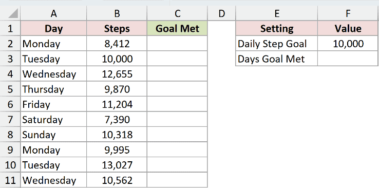
We want to flag every day that meets the 10,000-step goal, then count those days.
Enter this formula in C2 and copy it down through C11:
=GESTEP(B2,$F$2)
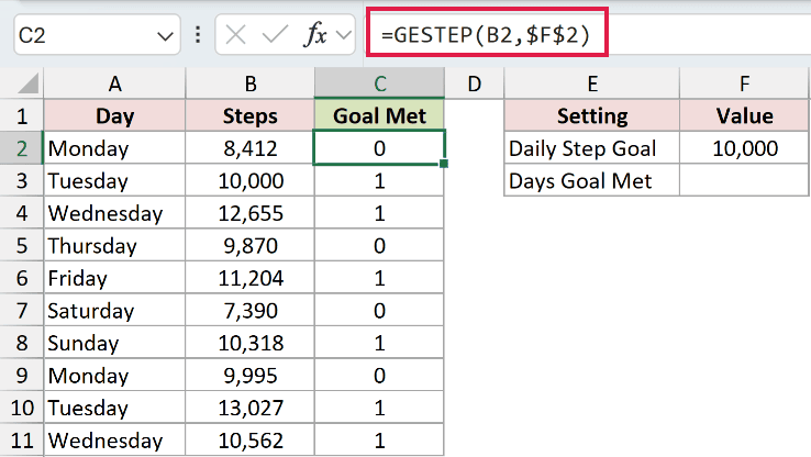
B2 changes as you copy down, while $F$2 keeps the goal fixed. The first Monday’s 8,412 steps return 0.
Tuesday’s 10,000 steps return 1 because reaching the goal exactly counts. The later Monday with 9,995 steps returns 0.
These are per-row formulas. Passing a bare range to GESTEP returns a single #VALUE! error. We’ll fix that in Example 5.
To count the qualifying days, enter this formula in F3:
=SUM(C2:C11)
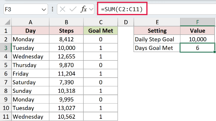
The result is 6. SUM adds the numeric flags, so each day that met the goal contributes to the count.
Pro Tip: COUNTIF can count values at or above a goal directly. Choose GESTEP when you also want a visible flag for each row, ready for another calculation.
Example 2: Calculate Incentives Against Individual Targets
Now each store has its own target, but the incentive amount stays fixed.
Below is the dataset. Columns A:C list stores, gift cards sold, and monthly targets. D will hold incentives; F:G contains the incentive input and total label.
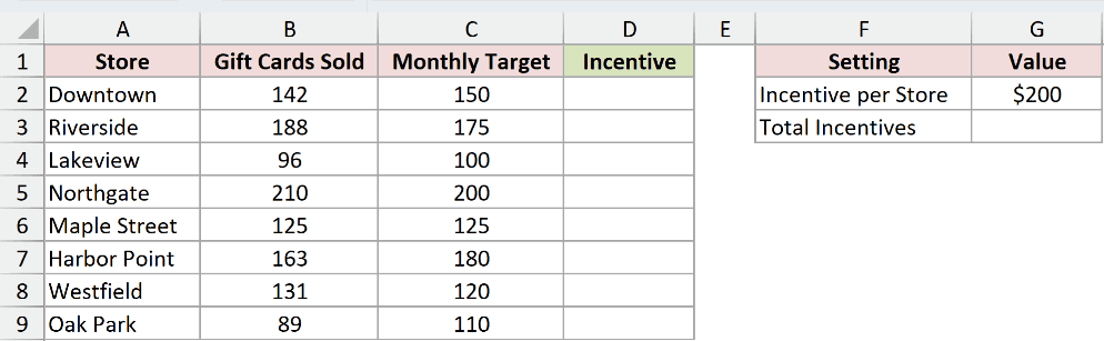
We want to pay $200 to each store that meets or exceeds its monthly target.
Enter this formula in D2 and copy it down through D9:
=GESTEP(B2,C2)*$G$2
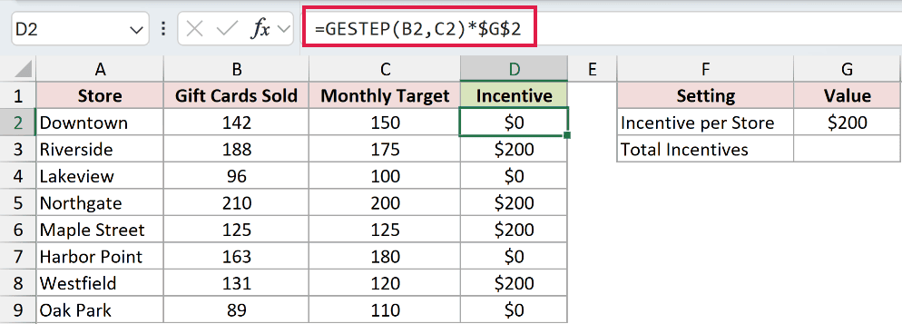
GESTEP compares the sales and target on the same row. Multiplying its numeric flag by the locked incentive amount turns the qualifying flag into a payment.
Downtown sold 142 gift cards against a target of 150, so its incentive is $0. Riverside sold 188 against 175 and receives $200.
Maple Street sold exactly 125 against a target of 125. Its $200 incentive confirms that matching the target qualifies too.
Enter the total incentive formula in G3:
=SUM(D2:D9)
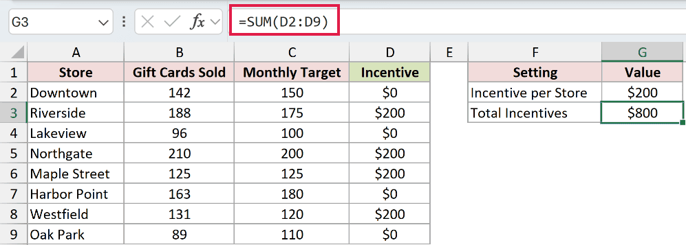
The total is $800. Riverside, Northgate, Maple Street, and Westfield qualify for the payment.
IF can express the same payment rule. GESTEP is useful here because its numeric result can be multiplied directly by the amount.
Example 3: Test Against the Default Zero Threshold
Leaving out step makes GESTEP useful for checking whether a change is nonnegative.
Below is the dataset. Columns A:B contain months and net subscriber changes. C will hold flags, and F2 will hold the count beside its label.
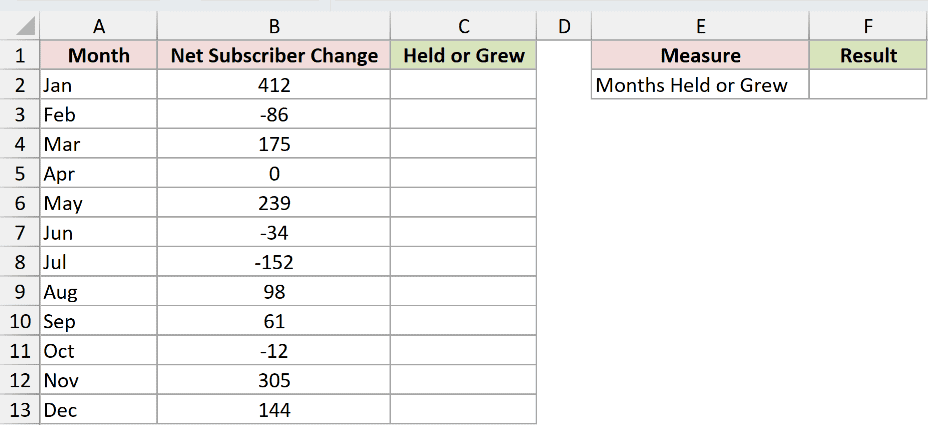
We want to identify months when the subscriber count held steady or grew.
Enter this formula in C2 and copy it down through C13:
=GESTEP(B2)
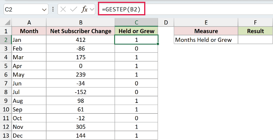
With no step argument, GESTEP compares each change with 0. January’s 412 returns 1, while February’s -86 returns 0.
April’s change is 0 and its flag is 1.
The column header says “Held or Grew”. This test includes months with no net change.
To count those months, enter this formula in F2:
=SUM(C2:C13)
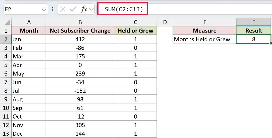
The result is 8. If you only want months with growth, use a strictly greater-than comparison instead of this inclusive test.
Example 4: Build Loyalty Tiers From Spending
Adding GESTEP checks together lets you count how many spending thresholds a customer has reached.
Below is the dataset. Columns A:B contain customers and annual spending. E:F lists tier names and minimum spending, while C will hold numeric tier levels.
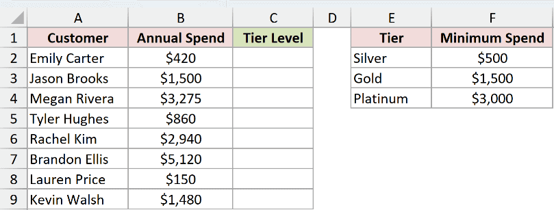
We want to assign a tier level based on the Silver, Gold, and Platinum spending thresholds.
Enter this formula in C2 and copy it down through C9:
=GESTEP(B2,$F$2)+GESTEP(B2,$F$3)+GESTEP(B2,$F$4)
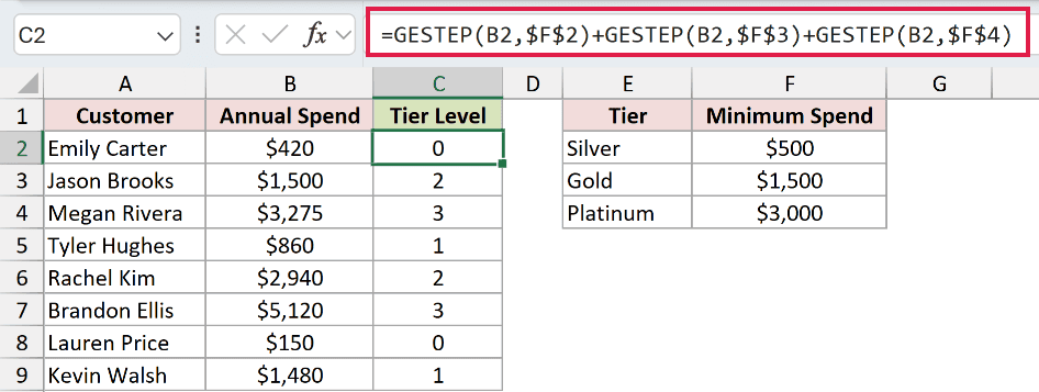
Each GESTEP checks the same spending amount against a different locked threshold. Adding the flags returns the number of thresholds met.
The levels correspond to these spending bands:
- 0: Below the $500 Silver threshold.
- 1: At least $500 but below the $1,500 Gold threshold.
- 2: At least $1,500 but below the $3,000 Platinum threshold.
- 3: At least $3,000.
Emily Carter’s $420 returns 0. Tyler Hughes’s $860 returns 1, while Megan Rivera’s $3,275 returns 3.
Jason Brooks spends exactly $1,500 and returns 2. He meets both the Silver and Gold thresholds, so his level is Gold.
This formula returns a numeric level. If you need the tier name directly, an approximate-match lookup can be easier to maintain as the tier list grows.
Example 5: Fix the GESTEP Range Error
GESTEP needs an extra step when you want to process an entire range in a single formula.
Below is the dataset. A:B lists bus runs and minutes late; C will hold flags. E:F contains the threshold, a deliberate error demonstration, and the corrected count label.
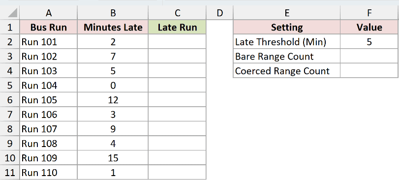
We want to flag and count bus runs arriving at least 5 minutes late.
Enter this formula in C2:
=GESTEP(+B2:B11,F2)
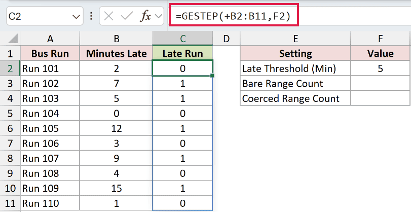
The leading + makes Excel evaluate the range as an array of values that GESTEP can process. The formula spills its flags into C2:C11.
Run 101 is 2 minutes late and returns 0. Run 103 is exactly 5 minutes late and returns 1.
This spill works in Excel 2021, Excel 2024, and Microsoft 365. In Excel 2019 and earlier, use per-row formulas copied down, as in the earlier examples.
The formula in F3 deliberately demonstrates the wrong way to count a bare range:
=SUM(GESTEP(B2:B11,F2))
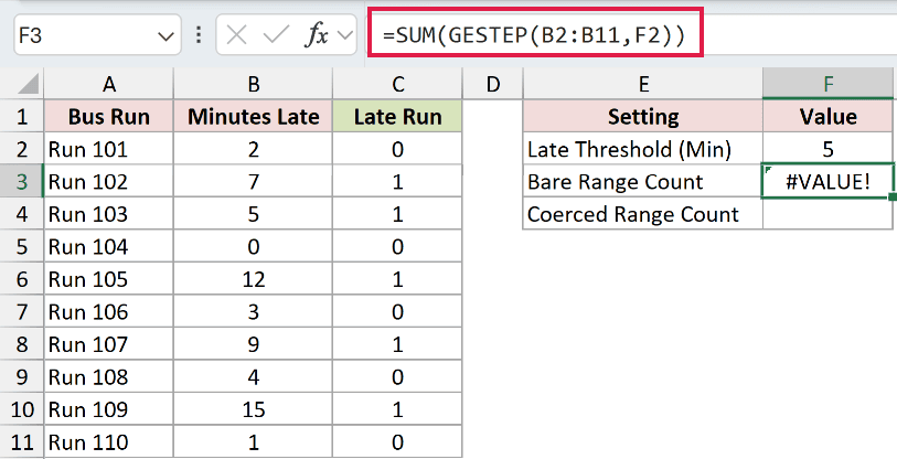
This deliberate mistake returns #VALUE!. GESTEP rejects the bare range before SUM can add anything, so wrapping it in SUM doesn’t solve the problem.
The corrected count in F4 adds the leading + inside GESTEP:
=SUM(GESTEP(+B2:B11,F2))
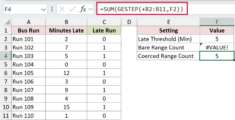
The corrected formula returns 5. GESTEP now processes the values, and SUM combines the resulting flags into a single count.
COUNTIF is the more direct choice if the count is all you need.
Tips & Common Mistakes
- GESTEP includes values equal to the threshold. Use a strict comparison when the requirement says “more than.”
- GESTEP accepts numbers stored as text, but nonnumeric text returns
#VALUE!. A logical input such as TRUE also returns#VALUE!. - A blank cell counts as 0. Decide whether missing readings should be included before applying a threshold test.
- A bare range in
stepalso returns#VALUE!. The per-row method lets each row reference its own threshold safely. - A greater-than-or-equal comparison converted to a number can produce the same flags. COUNTIF can count qualifying values without a helper column.
- DELTA tests numeric equality; GESTEP tests whether a number has reached a threshold.
Keep the threshold in a clearly labeled input cell when it may change. The flags and any totals based on them can then follow the updated rule.
You can use GESTEP flags to count targets met, calculate incentives, and assign loyalty tiers.
The examples also covered the default zero threshold and the range-input fix for counting several values in one formula.
Related Excel Functions / Articles:
