
Excel’s GETPIVOTDATA function returns a visible value from a PivotTable using field and item names.
It is useful for reports that must refer to a particular PivotTable result even when its position changes. The requested data must still be available in the PivotTable.
For a summary created directly by a formula, GROUPBY and PIVOTBY serve a different purpose: they aggregate the source data rather than retrieve an existing PivotTable result.
In this article, I’ll show you how to retrieve PivotTable totals, select values at row-column intersections, and make the requested item depend on a cell.
GETPIVOTDATA Function Syntax in Excel
Here’s the syntax:
=GETPIVOTDATA(data_field, pivot_table, [field1, item1], [field2, item2], ...)
- data_field: the name of the value field you want returned, as text in quotes. For a pivot with a single value column, this is usually the source column name like
"Sales". When the pivot has multiple value columns (Sum and Average, for instance), use the full displayed name like"Sum of Sales"or"Average of Sales". - pivot_table: any cell reference that sits inside the pivot table. Excel uses this to identify which pivot the formula refers to. The convention is to use the top-left cell of the pivot (
$A$3in this article’s examples). - field1, item1, … (optional): up to 126 field/item pairs that narrow the result down to a specific cell in the pivot. Without any pairs, the formula returns the grand total of the value field.
When to Use GETPIVOTDATA Function
A few practical scenarios where this function earns its keep:
- You’re building a dashboard or summary report that needs to pull specific numbers from a pivot table.
- You want a formula that survives if someone drags fields around the pivot or changes its layout.
- You need to reference pivot totals or sub-totals in other formulas (think KPI tiles or comparison cards).
- You want a cell-driven lookup against a pivot, where typing a different region or product name into one cell updates the result automatically.
Source Data Used in These Examples
All six examples below use the same underlying dataset. It’s a small sales log with 35 rows, covering four regions, five products, and a year of dates.
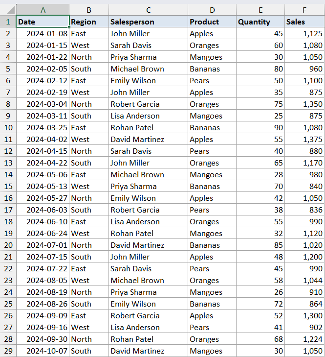
Each example sheet in the sample file has its own pivot table built from this data, shaped to suit what that example demonstrates.
Example 1: Pulling the Grand Total of Sales
Let’s start with the simplest case. The pivot here is a basic Region breakdown of Sales, with a Grand Total row at the bottom.
We want to pull the grand total of sales into a separate cell, outside the pivot.
Here is the formula:
=GETPIVOTDATA("Sales", $A$3)
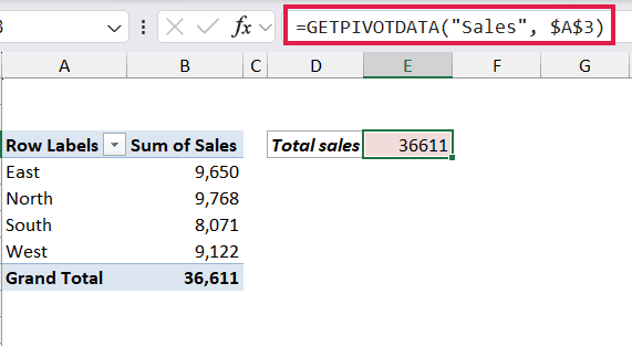
With just two arguments, the formula returns the overall grand total of the data field.
The first argument names the value field (Sales), and the second points at the pivot itself by referencing any cell inside it.
Pro Tip: If you type = and then click on the Grand Total cell inside a pivot, Excel does not return a plain cell reference. It writes a full GETPIVOTDATA formula for you. That is where most people first encounter this function.
Example 2: Pulling the Total for a Single Region
The pivot stays the same as the previous example. This time we want only the East region’s total, not the grand total.
Here is the formula:
=GETPIVOTDATA("Sales", $A$3, "Region", "East")
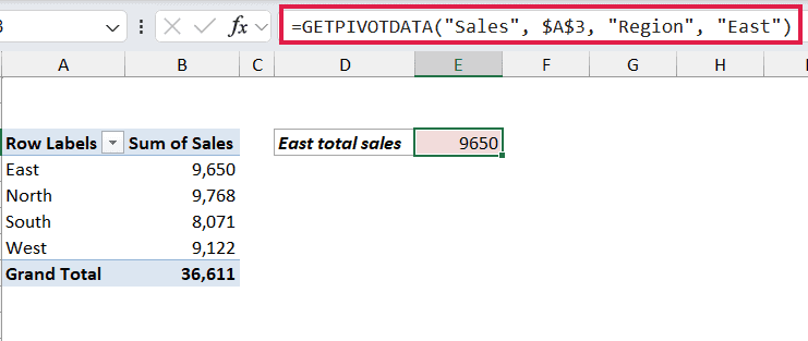
The new pair of arguments tells GETPIVOTDATA to narrow the result. "Region" is the field name (the column the pivot uses for rows), and "East" is the item we want from that field. The formula returns 9650, which matches the East row in the pivot.
You can keep stacking pairs to drill deeper. The next example does exactly that.
Example 3: Pulling a Value at a Row-Column Intersection
This example uses a richer pivot: Region as rows, Product as columns, and Sum of Sales as the values. We want one cell from that grid, the total of Apples sold in the West.
Here is the formula:
=GETPIVOTDATA("Sales", $A$3, "Region", "West", "Product", "Apples")
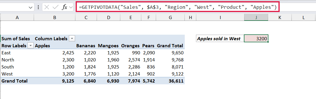
Two field/item pairs are doing the work here. The first pair narrows down to the West row, the second pair narrows to the Apples column, and the intersection of the two is the value the formula returns.
The order of the pairs doesn’t matter. ("Product", "Apples", "Region", "West") would return the exact same value. Excel matches each pair to the relevant pivot field by name.
Pro Tip: If you don’t have a pivot table set up, the SUMIFS function does this same job directly against the raw data: =SUMIFS(Sales[Sales], Sales[Region], "West", Sales[Product], "Apples"). GETPIVOTDATA is the right pick when you already have a pivot built for users to interact with; SUMIFS is the right pick when you’re starting from a clean data table.
Example 4: Making the Formula Dynamic with a Cell Reference
Hard-coding "East" or "West" in the formula is fine for static reports. But GETPIVOTDATA gets a lot more interesting when you point an item argument at a cell instead. The formula then updates as soon as you change the value in that cell.
In this sheet, cell E2 holds the region we want to look at. Cell E3 holds the formula. Change E2 from “South” to “North”, and the result updates instantly.
Here is the formula:
=GETPIVOTDATA("Sales", $A$3, "Region", E2)
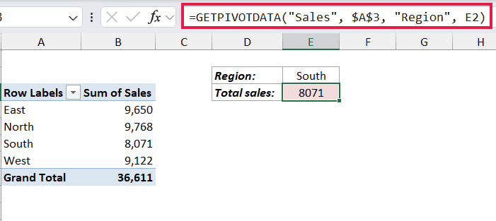
The fourth argument is now a cell reference instead of a string literal. Whatever text sits in E2 becomes the item GETPIVOTDATA looks up. This is the pattern you’ll use most often in dashboards: a dropdown in one cell, a GETPIVOTDATA formula reading from it in another.
Pro Tip: Pair the criterion cell with a data validation dropdown listing the valid items. The user picks from the list, the formula updates, and there is no risk of a typo turning the result into a #REF! error (see Example 6).
Example 5: Pulling the Average Instead of the Sum
So far every formula has pulled a sum. GETPIVOTDATA works for any value field the pivot exposes, not just sums.
This sheet’s pivot has two value fields: Sum of Sales and Average of Sales. We want the average for the South region.
Here is the formula:
=GETPIVOTDATA("Average of Sales", $A$3, "Region", "South")
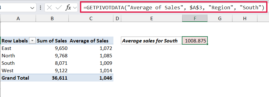
The change is in the first argument. With two value fields in the pivot, the source column name "Sales" alone is ambiguous, so we use the full displayed name "Average of Sales" instead. That is exactly the text shown in the pivot’s column header for the field.
If you ever rename a value field in the pivot (right-click the field, Value Field Settings, change the Custom Name), update the first argument of any GETPIVOTDATA formula referencing it.
The data_field argument must match the displayed name, not the source column. Same applies if you change the summary from Count to Sum or to any other aggregation. The displayed name changes, and GETPIVOTDATA has to follow.
Example 6: When the Item Doesn’t Exist
What happens when you ask GETPIVOTDATA for an item that isn’t in the pivot? The formula returns a #REF! error.
Here is a formula asking for the “Central” region, which doesn’t appear in our source data:
=GETPIVOTDATA("Sales", $A$3, "Region", "Central")
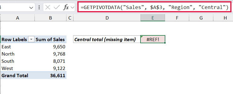
This is by design. GETPIVOTDATA can only return values that the pivot has computed, and the pivot only has rows for regions present in the data. There is no row for “Central”, so there is nothing for the formula to return.
The same error shows up if you misspell an item (“Eastt” instead of “East”) or reference a field name the pivot doesn’t have.
To make the formula safer when the criterion can vary, wrap it in IFERROR:
=IFERROR(GETPIVOTDATA("Sales", $A$3, "Region", E2), 0)
That way a missing item returns 0 (or any fallback you choose) instead of an error spreading through dependent formulas.
Tips & Common Mistakes
- Turn off the auto-generation if it gets in the way. When you type
=in a cell and click anywhere inside a pivot, Excel writes a full GETPIVOTDATA formula instead of a plain cell reference. If you’d rather get the cell reference, go to PivotTable Analyze > Options > and uncheck Generate GetPivotData. - The data field name must match the pivot’s displayed name when there are multiple value fields. “Sum of Sales” and “Average of Sales” are different fields to GETPIVOTDATA, even though they come from the same source column.
- The pivot_table argument can be any cell inside the pivot. Pointing it at
$A$3(the top-left) is the cleanest convention because that cell stays anchored to the pivot even if the data area expands. - Order of field/item pairs doesn’t matter. Excel matches each pair by field name, not by position.
- Grouped date fields become new field names. If you group the Date field into Years and Quarters, your formulas need to reference
"Years"and"Quarters", not"Date". - GETPIVOTDATA results only update when the pivot does. If the source data changes, you need to refresh the pivot table before the formula picks up the new numbers. Pivots don’t recalculate automatically the way regular formulas do.
- Modern alternative: GROUPBY and PIVOTBY in Excel 365 return pivot-style results as a single spilling formula. If you’re building a new dashboard from scratch, those two functions often remove the need for GETPIVOTDATA entirely. The function still matters for any workbook with an existing pivot you want to read from.
GETPIVOTDATA exists for one practical reason. Any formula that references a pivot cell directly will break the moment someone reorganizes the pivot. A GETPIVOTDATA formula keeps working. That’s why Excel auto-generates it when you click on a pivot in the first place.
The six examples above cover the patterns you’ll run into most often: pulling totals, narrowing with one or two criteria, going dynamic with a cell reference, switching to a different value field, and handling missing items. The Pro Tips and the gotchas in the Tips section are the things worth knowing before you put GETPIVOTDATA into a real workbook.
Related Excel Functions / Articles:
- How to Add Calculated Field to Pivot Table?
- Microsoft Excel Terminology (Glossary)
- How to Change Data Source in Pivot Table
- How to Delete a Pivot Table in Excel?
- How to Copy a Pivot Table in Excel?
- How to Clear Pivot Table Cache?
- How to Sum a Column in Excel?
- Remove Grand Total From Pivot Table in Excel
- Calculate differences inside a PivotTable
