
Excel’s MAX function returns the largest number in a set of values.
You can find the highest sale, latest date, or maximum across separate ranges. For the largest value meeting specific conditions, MAXIFS can apply those conditions directly.
In this article, I’ll show you how to find the latest date, calculate a maximum for one group, and return the highest value in each row.
MAX Function Syntax in Excel
Here is the syntax of the MAX function:
=MAX(number1, [number2], ...)
number1is the first number, cell, range, or array you want to evaluate. This argument is required.[number2]is an optional additional number, cell, range, or array. You can supply up to 255 arguments in total.
MAX returns the largest numeric value it finds. When you pass a cell range, it ignores blank cells, text, and logical values stored in that range.
When to Use MAX Function
Use MAX when you need to:
- Find the highest number in a column or row.
- Compare values stored in separate ranges.
- Return the latest date from a date list.
- Find the highest value that matches a condition.
- Calculate one maximum for every row of a table.
Example 1: Find the Highest Number in a Range
Let’s start with the most common way to find the largest value in Excel.
Below is a dataset with eight buildings in column A and their peak electricity demand in column B.
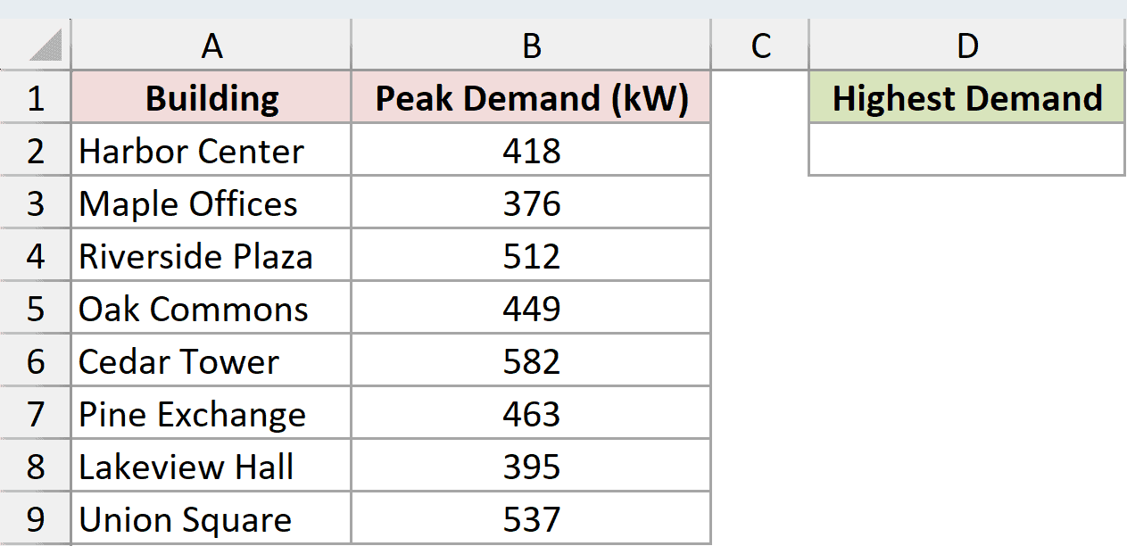
I want to return the highest demand reading in cell D2.
Here is the formula:
=MAX(B2:B9)
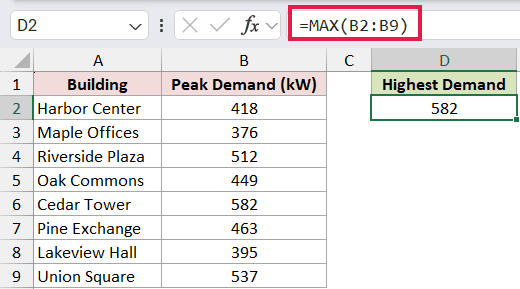
MAX checks every numeric value in B2:B9 and returns 582. That is the peak demand recorded for Cedar Tower.
The order of the rows does not matter. MAX always returns the largest numeric value in the supplied range.
Example 2: Find a Maximum Across Separate Ranges
You can also give MAX more than one range.
The dataset below has daily pallet volumes for the East Dock in column B and the West Dock in column D. Column C contains damaged-pallet counts that should not be included.
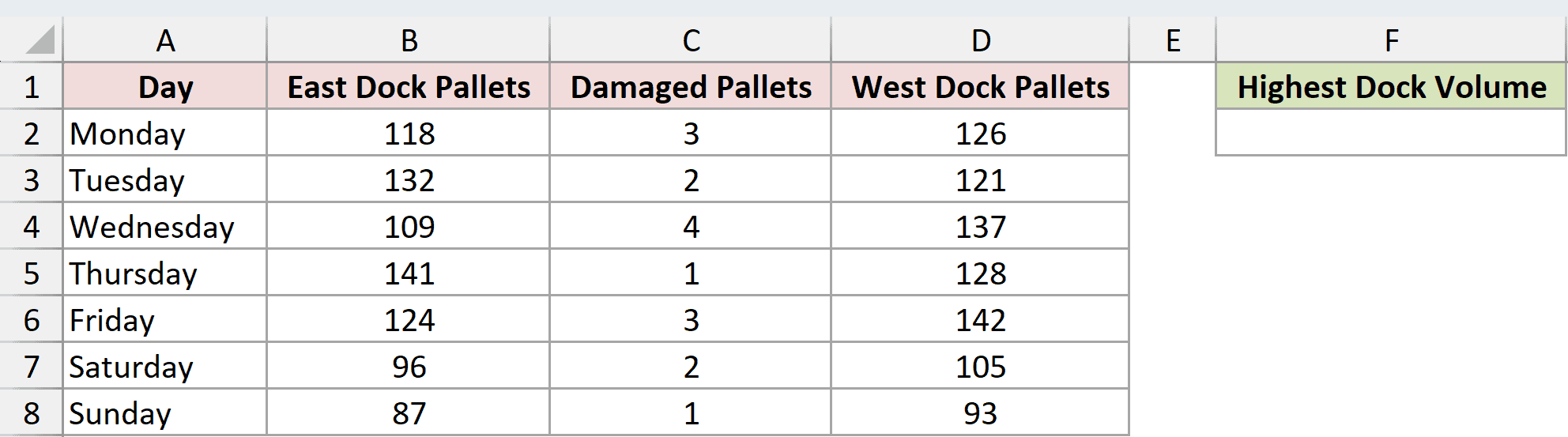
I want the highest dock volume from columns B and D without including column C.
Here is the formula:
=MAX(B2:B8,D2:D8)
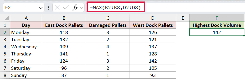
The two range arguments tell MAX exactly which cells to compare. It returns 142, the West Dock volume recorded on Friday.
Column C sits between the two ranges, but MAX never reads it because the formula does not include it.
Pro Tip: Separate each additional range or value with a comma. MAX accepts up to 255 arguments, so you do not need to combine nonadjacent ranges first.
Example 3: Use MAX to Find the Latest Date
MAX works with dates too.
Below is a vendor list with certificate-expiry dates in B2:B9.
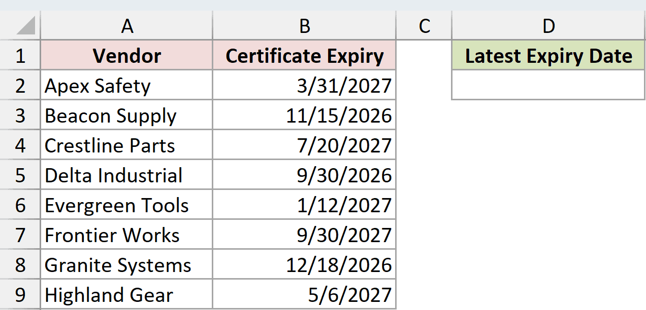
I want to find the latest certificate-expiry date in the list.
Here is the formula:
=MAX(B2:B9)
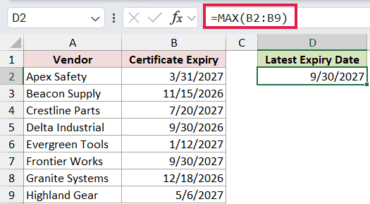
Excel stores dates as serial numbers, with later dates represented by larger numbers. MAX therefore returns 9/30/2027, the latest date in B2:B9.
Pro Tip: If the result appears as a number instead of a date, apply a date format to the result cell. The MAX formula itself does not need to change.
Example 4: Ignore Text and Blank Cells
Real worksheets often contain unfinished records or status notes alongside numbers.
This inspection log has numeric pressure readings in column B, plus the text entries Pending and Recheck and one blank cell.
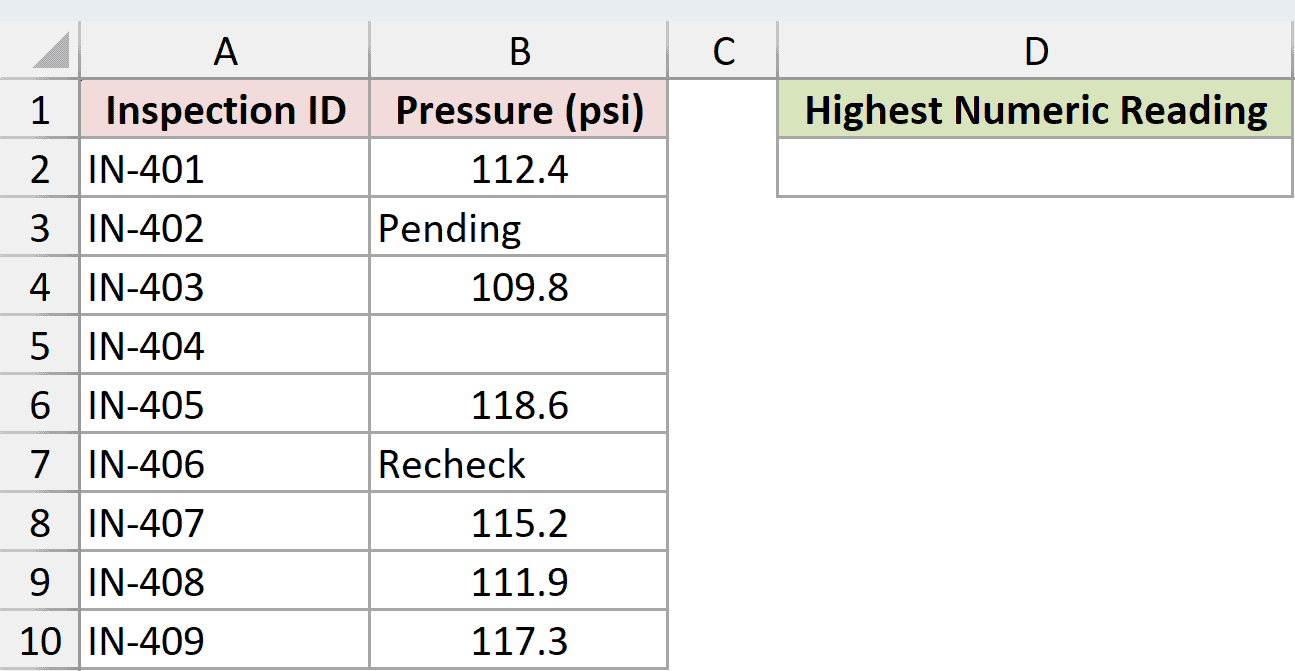
I want the highest completed numeric reading from B2:B10.
Here is the formula:
=MAX(B2:B10)
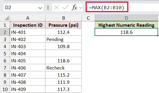
MAX ignores the text and blank cells in the referenced range. It evaluates the six numeric readings and returns 118.6 psi.
Zeros are different from blanks. A zero is a number, so MAX includes it in the comparison.
Pro Tip: MAX does not ignore error values. If a referenced cell contains an error, fix or handle that source value before calculating the maximum.
Example 5: Find a Conditional Maximum
Sometimes you need the highest value for one category rather than the entire list.
The dataset below contains repair jobs, their service types, and repair costs. Cell E2 contains the service type Emergency.
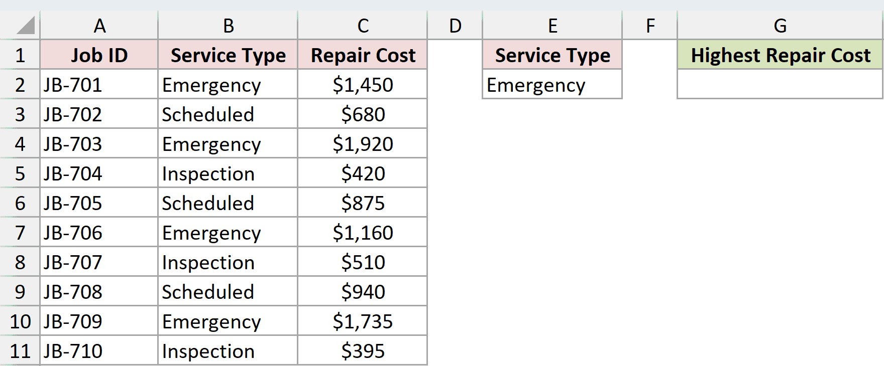
I want the highest repair cost among emergency jobs only.
Here is the formula:
=MAX(FILTER(C2:C11,B2:B11=E2))
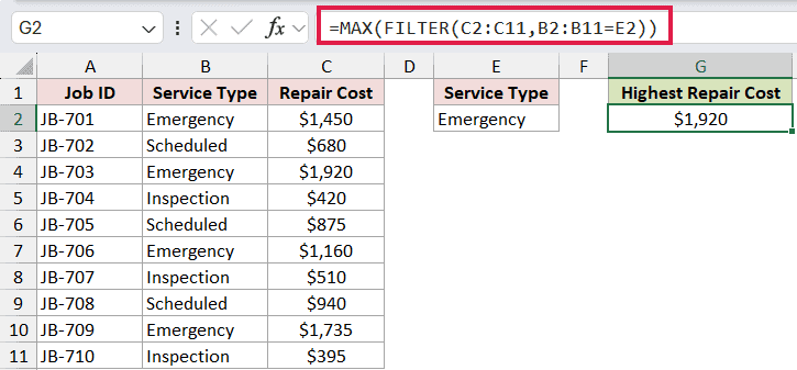
How this formula works:
B2:B11=E2checks which jobs have the Emergency service type.- FILTER returns only the matching repair costs.
- MAX returns the largest filtered cost, which is $1,920.
If the maximum and criteria ranges have matching dimensions, MAXIFS can do the same job with =MAXIFS(C2:C11,B2:B11,E2). The FILTER version is useful when the filtered array also feeds other calculations.
FILTER requires a dynamic-array version of Excel, including Microsoft 365, Excel 2024, or Excel 2021.
Example 6: Find the Maximum in Each Row
The last example returns several maximums with one formula.
This venue table has attendance for Friday, Saturday, and Sunday in columns B:D.
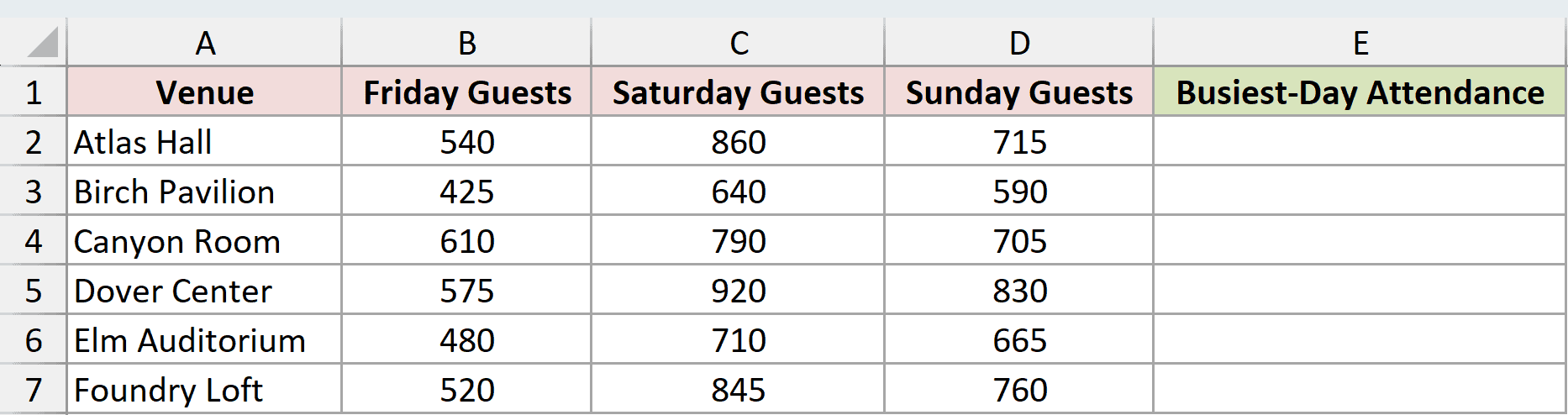
I want one busiest-day attendance figure for every venue.
Here is the formula:
=BYROW(B2:D7,LAMBDA(period,MAX(period)))
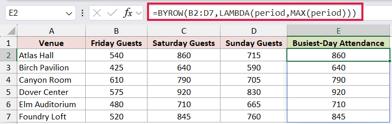
How this formula works:
BYROWpasses one row from B2:D7 to the LAMBDA at a time.periodis the name assigned to the current row.MAX(period)returns that row’s largest attendance figure.
The formula spills 860, 640, 790, 920, 710, and 845 into E2:E7. You do not need to copy a separate MAX formula down the column.
BYROW is available in Microsoft 365 and Excel 2024.
Tips & Common Mistakes
- MAX returns 0 when none of its arguments contain a number. Check the source range if that zero is unexpected.
- Text and logical values typed directly as formula arguments are treated differently from the same values stored in referenced cells. In a referenced range, MAX ignores them.
- Use MAXA when TRUE, FALSE, and text representations of numbers stored in references should take part in the calculation.
- MAX returns the largest value, not the position or full record containing it. Use a lookup or filtering formula when you need related information from the same row.
- MAX does not spill on its own because it reduces a range to one value. It can still consume spilled arrays and work inside formulas built with FILTER, BYROW, and other dynamic array functions.
I covered the standard MAX formula, separate ranges, dates, mixed data, a conditional maximum, and a row-by-row dynamic array calculation. I hope you found this article helpful.
Related Excel Functions / Articles:
