ROUNDUP Function in Excel

If you want to round numbers up to a fixed number of decimal places, or up to the next whole number, ten, or hundred, the ROUNDUP function in Excel is what you’re looking for.

Unlike the regular ROUND function, ROUNDUP always pushes the value up, no matter what the next digit is.

In Excel 365, you can also feed ROUNDUP a range of numbers and the results spill into the cells below.

In this article, I’ll walk you through how ROUNDUP works with a few practical examples.

ROUNDUP Syntax

Here is the syntax of the ROUNDUP function:

=ROUNDUP(number, num_digits)

• number – The number you want to round up.
• num_digits – The number of digits you want the result rounded to. Positive values round to the right of the decimal point, zero rounds to the nearest whole number, and negative values round to the left of the decimal point (tens, hundreds, thousands).

When to Use ROUNDUP

Use this function when you need to:

• Round prices, weights, or quantities up to a fixed number of decimal places.
• Round any value up to the nearest whole number so you never undercount.
• Round up to the nearest ten, hundred, or thousand for clean reporting.
• Calculate billable units (time blocks, shipping cartons, packaging) where partial units always count as a full unit.

Let me show you a few practical examples of how to use this function.

Example 1: Round Prices Up to Two Decimal Places

Let’s start with a simple example.

Below is the dataset with a list of product prices in column A. Each price has more than two decimal places, and I want to round each one up to exactly two decimals.

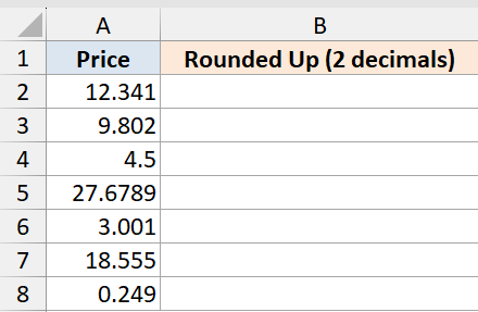
I want to round every price in the list up to two decimal places using a single formula.

Here is the formula:

=ROUNDUP(A2:A8,2)

In the above formula, I’m passing the entire range A2:A8 as the first argument. Since ROUNDUP spills in Excel 365, one formula in cell B2 fills all seven results down the column. The second argument, 2, tells ROUNDUP to keep two decimal places, always rounding the third decimal up.

So 12.341 becomes 12.35, and 9.802 becomes 9.81. Even values like 4.500 get pushed up to 4.50 (no change visually, but ROUNDUP is still applying its rule).

Pro Tip: If you’re on Excel 2019 or earlier, you’ll need to put =ROUNDUP(A2, 2) in B2 and drag it down. The spill behavior only works in Excel 365 and Excel for the web.

Example 2: Round Up to the Nearest Whole Number

Here’s another practical scenario.

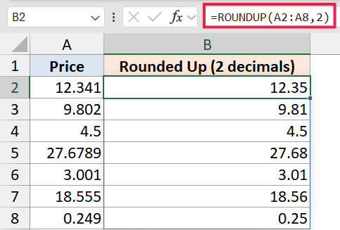
Below is a dataset showing the average daily steps walked by a few people over a week. The numbers come with decimals, but for a report card I want each value rounded up to the next whole step.

I want to round each daily step count up to the next whole number.

Here is the formula:

=ROUNDUP(B2:B7,0)

When the second argument is 0, ROUNDUP rounds the value up to the nearest integer. So 7234.2 becomes 7235, and 5108.9 becomes 5109. Even something tiny like 4001.01 still rounds up to 4002, since ROUNDUP doesn’t care how small the remainder is.

This is different from ROUND, which would have left 7234.2 as 7234. ROUNDUP always rounds away from zero.

Example 3: Round Up to the Nearest Ten or Hundred

Now let’s look at something a bit more interesting.

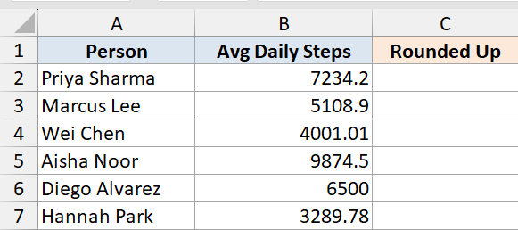
Below is a dataset of sales figures, and I want to round each value up to the nearest hundred so the numbers look cleaner in a summary slide.

I want to round each sales figure up to the next multiple of 100.

Here is the formula:

=ROUNDUP(B2:B7,-2)

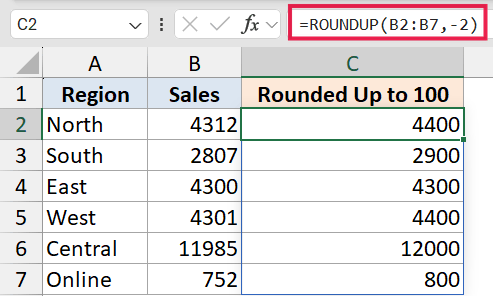
A negative num_digits tells ROUNDUP to round to the left of the decimal point.

• -1 rounds up to the nearest 10
• -2 rounds up to the nearest 100
• -3 rounds up to the nearest 1000

So 4312 becomes 4400, and 2807 becomes 2900. Even a value like 4300 stays at 4300, since it’s already a clean multiple of 100. But 4301 jumps to 4400 immediately, because ROUNDUP never leaves anything below the threshold.

This is handy when you want presentation-friendly numbers for forecasting or pricing tiers.

Example 4: Round Up Billable Hours to the Next 15-Minute Block

Let’s step it up with a more practical use case.

Below is a list of consulting sessions with the exact duration in hours (so 1.27 hours means 1 hour and roughly 16 minutes). For billing, I round every session up to the next quarter hour. A 16-minute session bills as 30 minutes, a 31-minute session bills as 45 minutes, and so on.

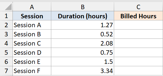
I want to round each session duration up to the next 0.25-hour block.

Here is the formula:

=ROUNDUP(B2:B7*4,0)/4

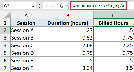
How this formula works:

• Multiplying the duration by 4 converts hours into “quarter-hour units” (1.27 hours becomes 5.08 quarter-hours).
• ROUNDUP with num_digits = 0 rounds that up to the next whole quarter (5.08 becomes 6).
• Dividing by 4 converts it back to hours (6 / 4 = 1.5 hours).

So a 1.27-hour session bills at 1.5 hours, and a 0.52-hour session bills at 0.75 hours. This trick of “multiply, round, divide” is the standard way to round up to any fixed interval. There’s a more direct approach using CEILING.MATH if you want to round time to the nearest quarter hour directly.

Pro Tip: If you’re rounding to multiples of 5 instead of 0.25, swap the 4 for 0.2 (so multiply by 0.2 and divide by 0.2 at the end). Or use =CEILING.MATH(B2, 5), which does the same thing in one shot. The same idea works for rounding up or down to the nearest 5.

Example 5: Calculate Boxes Needed to Pack Items

Here’s one more example I find genuinely useful.

Below is an order list. Each row has an order number and the quantity of items in that order. The items ship in boxes of 12, and I want to know how many boxes each order needs. A partial box still counts as a full box.

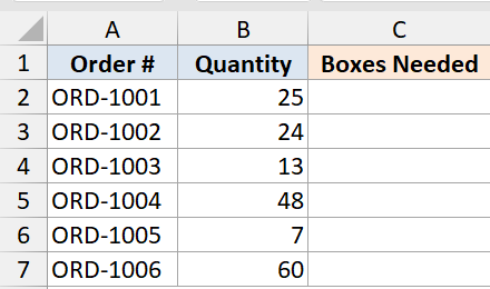
I want to calculate how many shipping boxes each order needs, where any partial box still counts as one full box.

Here is the formula:

=ROUNDUP(B2:B7/12,0)

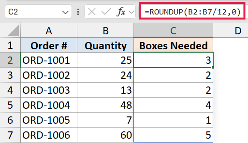
Dividing the quantity by 12 gives the exact number of boxes needed (so 25 items would mean 2.083 boxes). ROUNDUP with num_digits = 0 pushes that up to the next whole number, giving 3 boxes.

An order of 24 items stays at 2 boxes (since 24/12 = 2 exactly), but an order of 25 immediately jumps to 3. This is exactly the behavior you want for packaging, shipping, and any other “always round up to the next full unit” scenario.

Tips & Common Mistakes

• ROUNDUP always rounds away from zero, even for negative numbers. So =ROUNDUP(-2.3, 0) returns -3, not -2. If you want negative numbers to round toward zero, use ROUNDDOWN instead.
• Don’t confuse ROUNDUP with ROUND. ROUND uses standard rounding rules (so 2.4 rounds to 2 and 2.6 rounds to 3). ROUNDUP doesn’t care about the digit value, it always rounds up.
• For rounding up to a non-decimal interval, use CEILING.MATH instead. If you want to round up to the next multiple of 5, 25, or 100, =CEILING.MATH(A2, 5) is more direct than the “multiply, round, divide” trick with ROUNDUP. Both work, but CEILING.MATH reads more cleanly. If you just want to drop the decimals entirely without rounding up, see how to remove decimals in Excel.
• In Excel 2019 and earlier, you can’t pass a range to ROUNDUP and get a spilled result. You’ll need a per-cell formula filled down. In Excel 365 and Excel for the web, the spill works natively.
• Watch out for #SPILL! errors. If the spill range has values in any of the cells below the formula, Excel can’t spill into them. Clear the blocking cells and the formula will work.

ROUNDUP is one of those small functions that quietly solves a lot of real-world rounding problems. Whenever you need a number pushed up to the next decimal, the next whole number, or the next multiple of something, ROUNDUP is the cleanest tool for the job. Pair it with ROUND and ROUNDDOWN and you’ve got all the rounding behavior Excel has to offer.

List of All Excel Functions