Let’s face it, opening a worksheet to see decimals all over it can be quite off-putting. Some people find it intimidating, as decimals give the perception of complexity.
As such, one might sometimes need to remove decimals from numbers and turn them into whole numbers.
Excel provides a wide range of functions and options to help you remove decimals from numbers. In this tutorial we are going to look at some of these methods:
- Removing Decimals without Rounding
- Removing Decimals with Rounding
- Using Number Formatting to Remove Decimals
Removing Decimals without Rounding
If you simply want to convert a decimal value to a whole number, without rounding off, you can use the TRUNC function.
The TRUNC function takes a decimal value and truncates it to a given precision. So you can use it to truncate a number based on a given number of digits.
The syntax for the TRUNC function is as follows:
=TRUNC (number, [num_digits])
Here,
- number is numerical value or cell reference containing the number that you want to truncate.
- num_digits is the precision of the truncation. This value is optional, with a default value of 0.
If you want to extract just the integer part of a number by truncating (or removing) the fractional part, you can choose to ignore the second optional argument.
So, the function TRUNC(4.7) will return the value 4, while the function TRUNC(2.2) will return the value 2.
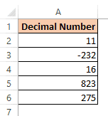
The following screenshot shows how the TRUNC function works with different decimal inputs:

Also read: How to Remove the Last Digit in Excel?
Removing Decimals by Rounding
If you would also like to round off the decimal number while removing it, there are a number of functions that Excel offers for this:
- INT
- ROUND
- ROUNDUP
- ROUNDDOWN
Let us take a look at each of these functions one by one to understand how they round off decimal values.
The INT Function
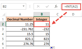
The INT function takes a decimal value and returns the integer part of it after rounding it down to the nearest integer. This means applying the function to both 10.8 and 10.2 will return the value 10.
The syntax for the INT function is simple:
=INT (number)
The function takes just one argument, which is the decimal number that needs to be converted to integer.
So, the function INT(4.7) will return the value 4, while the function INT(2.2) will return the value 2. Notice that this is the same result as the one we got from using the TRUNC function.
In fact, TRUNC and INT are both quite similar functions.
Similarities and Differences between TRUNC and INT
Both TRUNC and INT return the integer part of a number.
The main difference between them is that TRUNC simply truncates the decimal part while INT rounds the number down.
So applying the functions to positive numbers gives the same results.
However, they work differently on negative numbers. For example, while INT(10.8) returns 10, INT(-10.8) returns -11.
In other words, negative numbers become more negative when the INT function is applied to it.
This does not happen in the case of the TRUNC function. So, TRUNC(10.8) returns 10, while TRUNC(-10.8) returns -10.
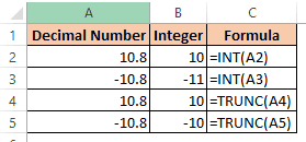
The following screenshot shows how the INT function works with different decimal inputs:
The general rule of thumb is:
- Use INT when you want the integer part of a decimal number, and you have no problem if it always rounds down.
- Use TRUNC if you want exactly the integer part of both negative and positive numbers.
Other Rounding Functions
The INT function’s main job is to round down a decimal number to its nearest integer, keywords here being, ‘rounding down’.
However, if you want more control over how you round off your decimal numbers, there is an arsenal of other functions provided by Excel.
Let’s take a look at some of these.
The ROUND Function
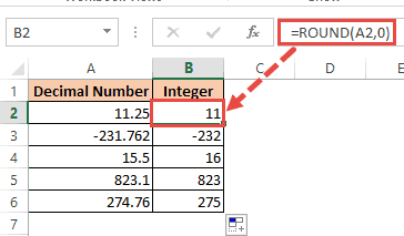
The ROUND function takes a decimal value and returns the number rounded to a given number of digits.
This function is capable of rounding down or up depending on the nearest number.
This means applying the function to 10.8 will return 11, while applying it to 10.2 will return 10.
The syntax for the ROUND function is as follows:
=ROUND (number, num_digits)
Here,
- number is numerical value or cell reference containing the number that you want to round.
- num_digits is the number of digits to which you want to round. This value is optional, with a default value of 0.
If you want to round the number to the nearest integer, you can set the num_digits argument to 0.
The following screenshot shows how the ROUND function works with different decimal inputs:
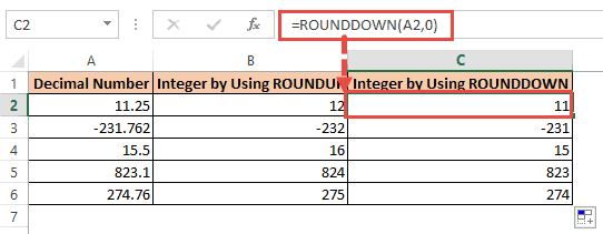
The ROUNDUP and ROUNDDOWN Functions
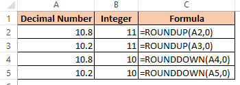
The ROUNDUP function takes a decimal value and returns the number rounded up to a given number of digits. This means applying the function to both 10.8 and 10.2 will return 11.
Conversely, The ROUNDDOWN function takes a decimal value and returns the number rounded down to a given number of digits. This means applying the function to both 10.8 and 10.2 will return 10.
The syntax for the ROUNDUP and ROUNDDOWN functions are the same as the ROUND function:
- =ROUNDUP (number, num_digits)
- =ROUNDDOWN (number, num_digits)
As before, if you want to round the number (up or down) to the nearest integer, you can set the num_digits argument to 0.
The following screenshot shows how the ROUNDUP and ROUNDDOWN functions work with different decimal inputs:
Also read: How to Round to Nearest 100 in Excel?
Removing Decimal with the Format Cells Dialog Box
If you only want to format the cells containing decimal values by removing the decimals (without actually affecting the original values in the cells), you can use the ‘Format Cells’ feature provided by Excel.
Here are the steps you need to follow:
- Select the cells containing the numbers you want to work with.
- Right-click on your selection and click on ‘Format Cells’ from the context menu that appears.
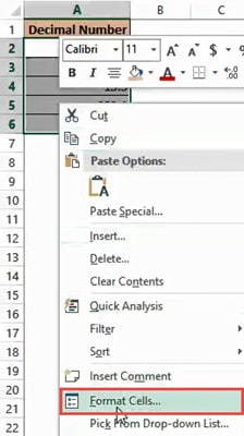
- This will open the Format Cells dialog box.
- Select the Number tab.
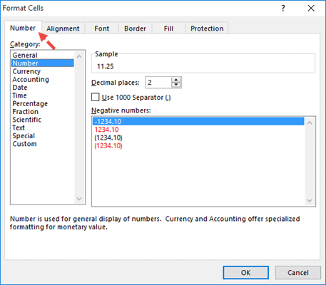
- Select the Number option from the list under ‘Category’.

- On the right side, next to Decimal places, bring the counter down to 0.
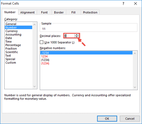
- Click OK to close the dialog box.
Your selected numbers should now be rounded to their nearest integers.
Notes:
- Using this method rounds the number up or down to the nearest integer, depending on the value after the decimal. In this way, it works somewhat like the ROUND function.
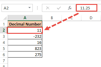
- This method only changes how the values in the cells look. It does not change the underlying values in the cells. So if you click on the cells, you would still be able to see the original (decimal) numbers in the formula bar.
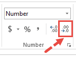
Alternatively, here’s a shortcut for this method. In the Number group, under the Home tab, you will find a ‘Decrease decimal’ button.
You can click this button to reduce the number of decimal places until all your numbers have turned into integers.
In this tutorial, we showed you multiple ways to remove decimals in Excel.
This included the use of functions to truncate, round up as well as round down your decimal numbers, to convert them into integers. We hope you found this tutorial useful.
Other articles you may also like:
- How to Convert Decimal to Fraction in Excel
- How to Apply Accounting Number Format in Excel
- How to Remove Leading Zeros in Excel
- How to Convert Serial Numbers to Date in Excel
- How to Convert Decimal to Binary in Excel
- Round UP or DOWN to Nearest 5 in Excel
- How to Change Commas to Decimal Points in Excel?