
The SKEW.P function in Excel returns population skewness, a measure of how unevenly a complete group’s values extend toward the high or low end.
A positive result points toward a longer high-value tail. A negative result points toward a longer low-value tail, such as a class with mostly high scores and occasional low scores.
Use SKEW.P when your records cover the whole group you’re describing. That could mean every student in a class or every shipment sent during a particular week.
I’ll show you how to interpret population skewness, calculate it separately for groups, and catch imported numbers that Excel silently leaves out.
SKEW.P Function Syntax in Excel
Pass SKEW.P the numbers or ranges you want to describe:
=SKEW.P(number1, [number2], ...)
- number1 (required): The first number, range, or array containing your data.
- number2, … (optional): Additional numbers, ranges, or arrays to include in the same calculation.
SKEW.P needs at least 3 numeric values, and they can’t all be identical. Otherwise, it returns #DIV/0!.
Text, logical values, and empty cells inside a range are skipped. That includes numbers stored as text, which can change the answer without producing an error.
When to Use SKEW.P Function
- Describe the shape of quiz scores for an entire class.
- Compare the asymmetry of different measurements across all orders in a reporting period.
- Calculate separate population-skewness results for complete groups within a sales list.
- Analyze all shipment weights for a week after checking that imported weights are numeric.
Example 1: Interpret a Complete Class’s Skewness
Let’s start with quiz scores for the whole class.
Below is the dataset. Column A lists students, column B holds quiz scores, and D2 will hold the population-skewness result.
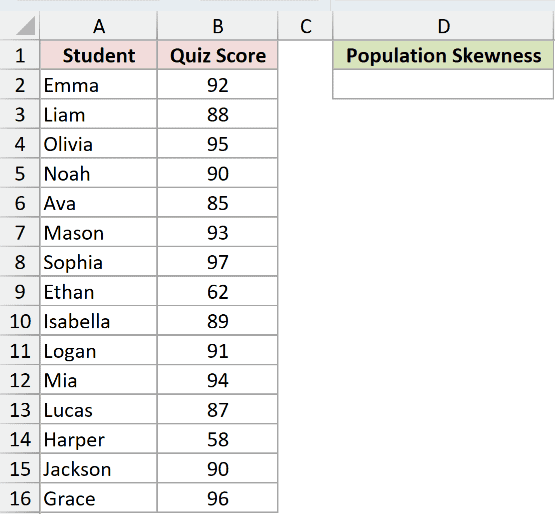
We want to measure which end of the class’s score distribution has the longer tail.
Enter this formula in D2:
=SKEW.P(B2:B16)
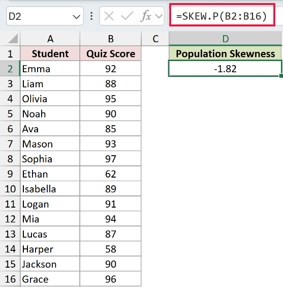
The result displays as -1.82. The negative sign indicates left skew: the scores extend farther toward the low end.
Most scores are clustered near the high end, while Ethan’s 62 and Harper’s 58 stretch the lower tail. Negative skewness doesn’t mean the scores themselves are negative.
SKEW.P summarizes the entire range in a single cell. It doesn’t spill a separate answer for each student, and it’s available in Excel 2013 and later.
Example 2: Compare Population and Sample Skewness
Now let’s see why the population-versus-sample choice changes the result on the same data.
Below is the dataset. Columns A and B list every store and its weekly returns; the labeled cells in D:E will compare population and sample calculations.
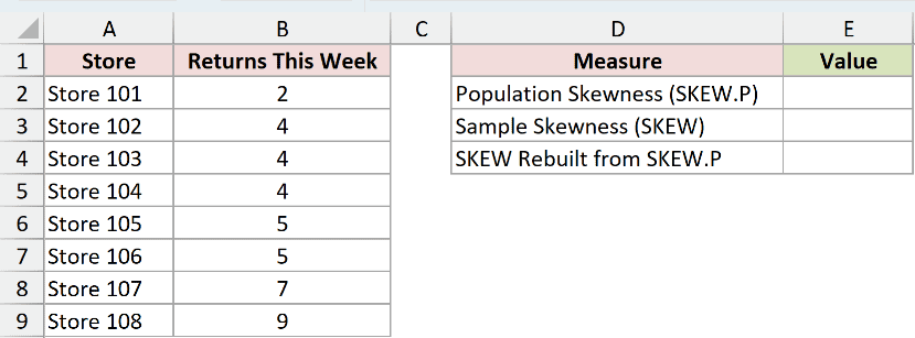
We want the population result for the complete store group, then a comparison showing the sample adjustment.
Enter the population formula in E2:
=SKEW.P(B2:B9)
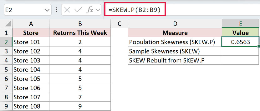
E2 displays 0.6563. This is the appropriate result when we’re describing all the stores in this group for this week.
For comparison, SKEW calculates sample skewness. It applies an adjustment when the observed stores are a sample used to describe a wider population.
Enter the sample comparison in E3:
=SKEW(B2:B9)
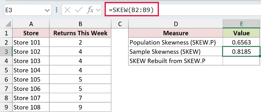
The sample skewness displays 0.8185. The sample adjustment increases the magnitude.
We can rebuild that sample comparison from the population result. COUNT counts the numeric observations, while SQRT takes the square root needed for the adjustment.
Enter the conversion comparison in E4:
=E2*SQRT(COUNT(B2:B9)*(COUNT(B2:B9)-1))/(COUNT(B2:B9)-2)
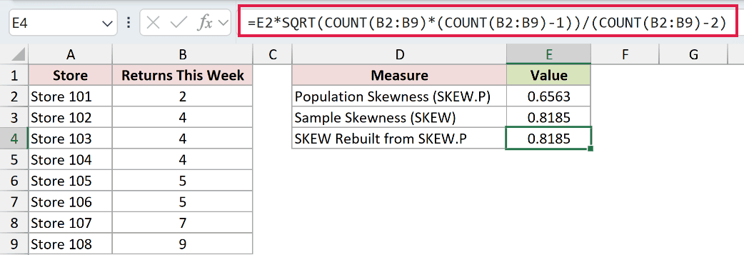
The rebuilt comparison also displays 0.8185, matching the sample formula.
The calculation multiplies E2 by an adjustment based on the observation count. Referencing E2 preserves its underlying precision instead of using the rounded value you see.
Pro Tip: Decide what group your conclusion describes before choosing the calculation. A complete list for this week’s stores can still be a sample if you’re trying to describe stores or weeks outside that list.
Example 3: Compare Dollars and Item Counts
Skewness lets us compare distribution shapes even when the measurements use different units.
Below is the dataset. Columns A:C contain every June order, its value, and item count; F2:G2 will hold the side-by-side skewness comparison.
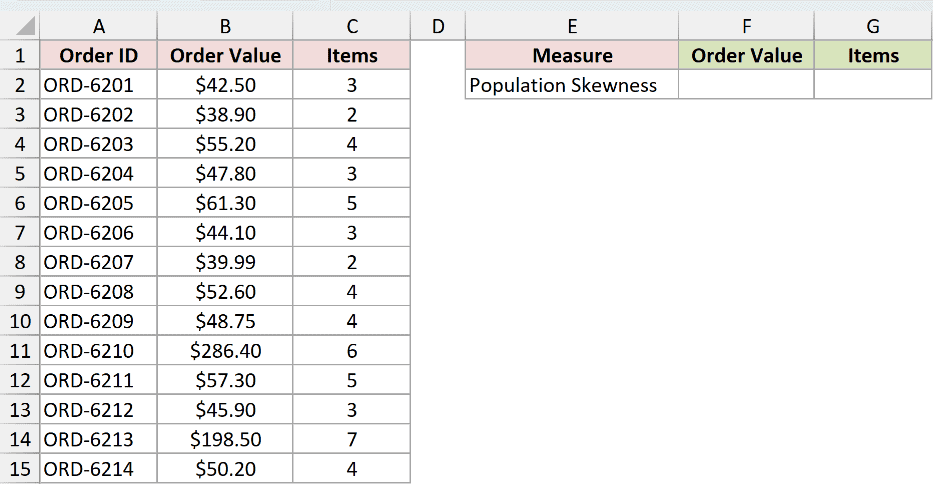
We want to compare the asymmetry of order values with the asymmetry of item counts across this complete month’s orders.
Start with the order-value result in F2:
=SKEW.P(B2:B15)
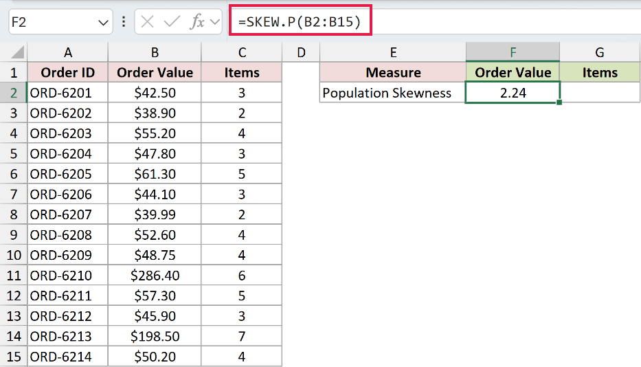
The order-value skewness displays as 2.24. Orders of $286.40 and $198.50 extend the high-value tail beyond the smaller orders.
For the item-count skewness, enter this formula in G2:
=SKEW.P(C2:C15)
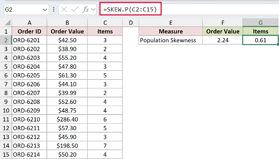
The item-count skewness displays 0.61. Both measures have positive skewness, but order values show greater positive asymmetry than item counts.
Both skewness results are unit-free measures of distribution shape.
Converting dollars to cents would leave the skewness unchanged. Multiplying all observations by the same positive factor changes their size, but preserves their relative shape.
Example 4: Calculate Skewness for Each Neighborhood
A complete sales list can contain groups with very different shapes.
Below is the dataset. Columns A:B list every sale in the reporting year by neighborhood, with prices in thousands; D:F provides neighborhood labels and result columns.
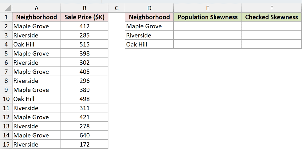
We want population skewness for each neighborhood, with a clear message where too few sales make the calculation impossible.
FILTER selects the prices belonging to the neighborhood named in D2. SKEW.P then calculates skewness from that selected group.
Enter this formula in E2 and copy it down through E4:
=SKEW.P(FILTER($B$2:$B$15,$A$2:$A$15=D2))
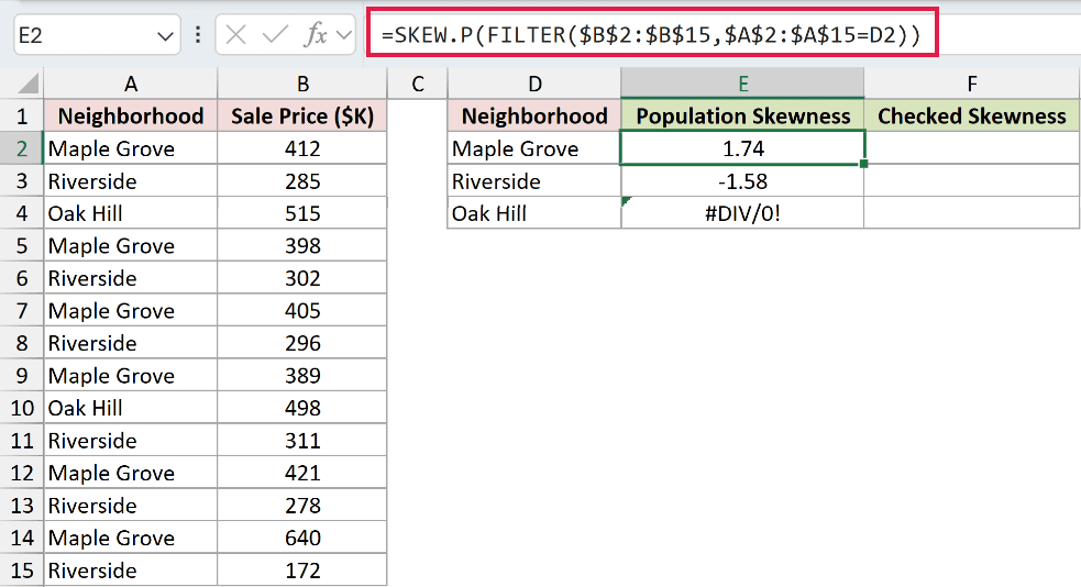
Maple Grove displays 1.74, while Riverside displays -1.58. Their sale-price distributions extend toward opposite ends: higher prices for Maple Grove and lower prices for Riverside.
Oak Hill deliberately shows #DIV/0! in E4. Its group has fewer than 3 sales, so this cell demonstrates the minimum-data error.
The dollar signs keep the source ranges fixed as D2 changes during copying. Filling down calculates one skewness result per neighborhood.
This FILTER combination needs Excel 2021, Excel 2024, or Microsoft 365.
To handle the small-group case, COUNTIF counts rows matching the neighborhood. IF checks that count and chooses either an explanatory message or the skewness calculation.
Enter the checked version in F2 and copy it down through F4:
=IF(COUNTIF($A$2:$A$15,D2)<3,"Need 3+ sales",SKEW.P(FILTER($B$2:$B$15,$A$2:$A$15=D2)))
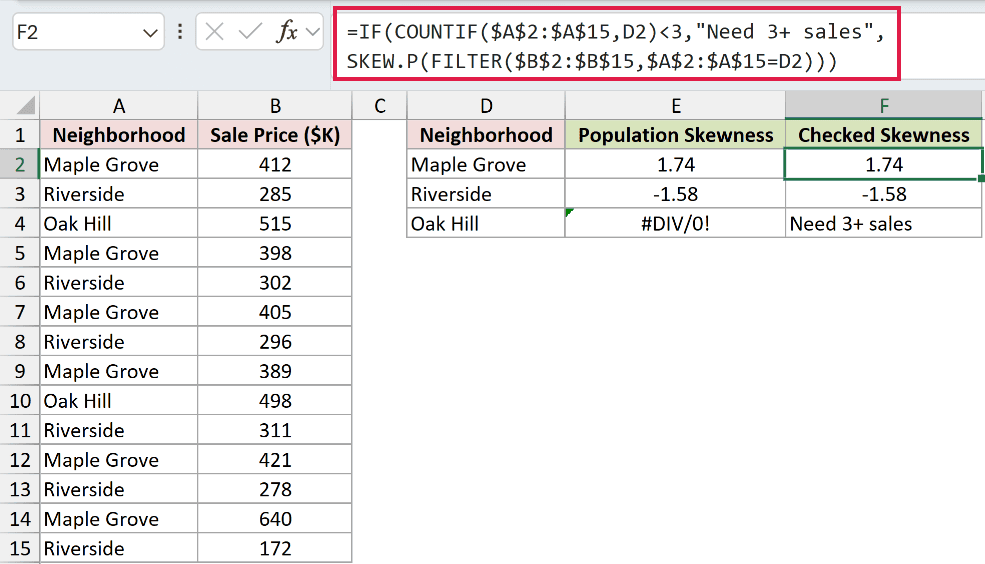
The Checked Skewness column retains 1.74 and -1.58, while F4 displays Need 3+ sales instead of the deliberate error in E4.
Pro Tip: This check counts matching sales rows, so it assumes their prices are numeric. It also doesn’t check for identical prices. SKEW.P still returns #DIV/0! when every included price is the same.
Example 5: Fix Numbers Stored as Text
Imported weights can look complete while SKEW.P quietly skips some shipments.
Below is the dataset. Columns A:B list every shipment from last week and its weight. D:F contains the As Imported and Text Converted results.
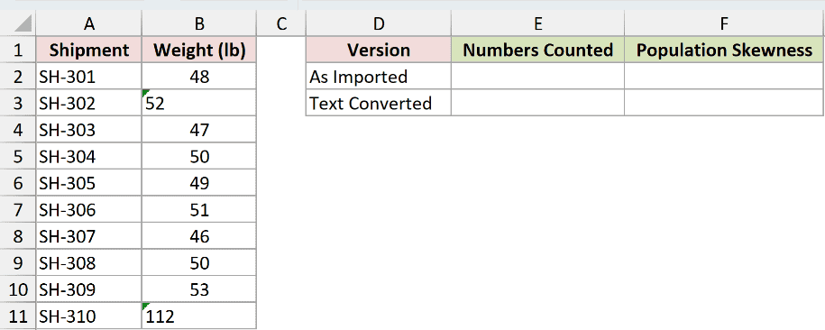
We want skewness for every shipment, including weights that arrived as text.
The weights 52 in B3 and 112 in B11 are stored as text. COUNT counts numeric cells, so it helps reveal what the as-imported calculation will include.
Enter the numeric count for the As Imported row in E2:
=COUNT(B2:B11)
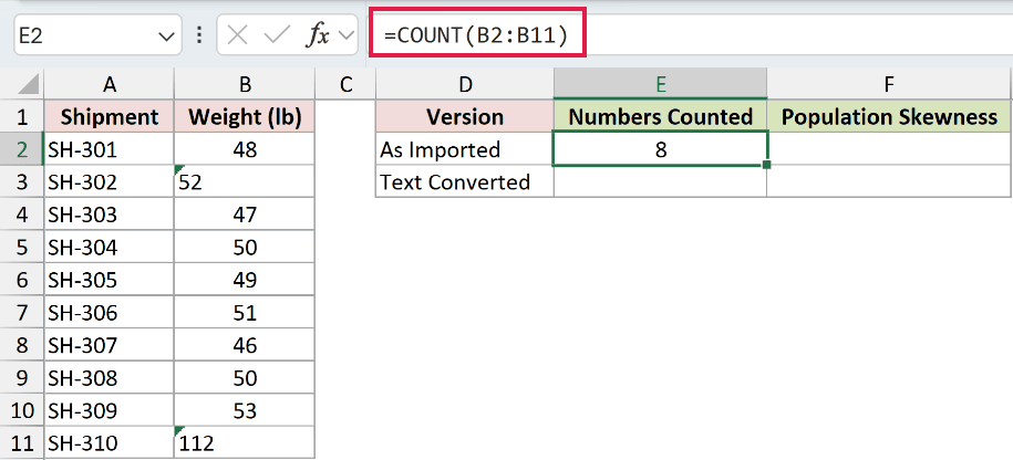
The As Imported count returns 8. The text weights don’t count as numbers, even though they look like weights on the sheet.
Enter the As Imported skewness formula in F2:
=SKEW.P(B2:B11)
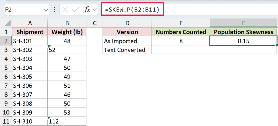
The As Imported skewness displays 0.15 without an error. It’s misleading for the full shipment group because the text weights were left out.
VALUE converts text that represents a number into a numeric value. Applying it to the weight range lets the calculation include the imported text weights.
Enter the numeric count for the Text Converted row in E3:
=COUNT(VALUE(B2:B11))
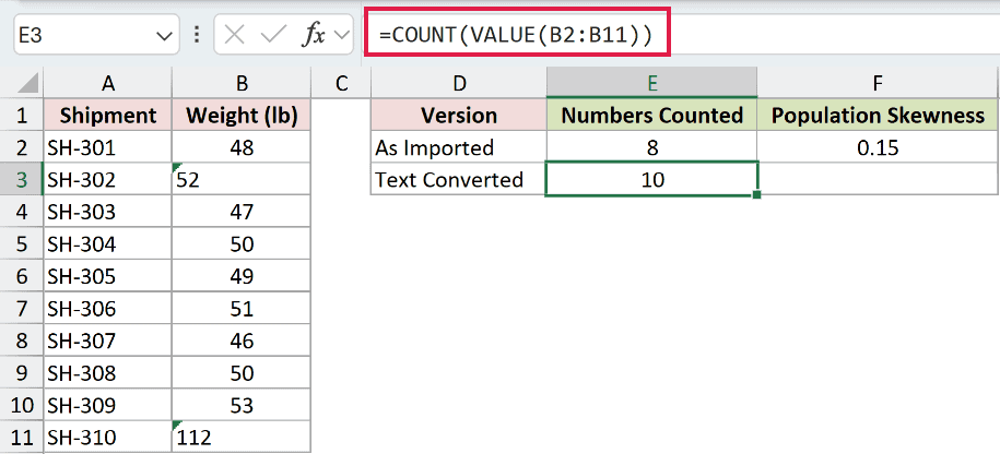
The Text Converted count returns 10, confirming that all shipment weights now participate in the calculation.
Enter the Text Converted population-skewness formula in F3:
=SKEW.P(VALUE(B2:B11))
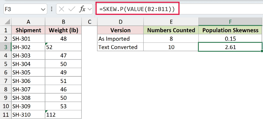
The Text Converted skewness displays 2.61. Including the 112-pound shipment reveals the high-weight tail missing from the As Imported result.
These range-based conversions need Excel 2021 or later. The outer functions return single results, and the conversion happens inside the formulas without changing the source cells.
Tips & Common Mistakes
- Define the complete group. A full list for a particular period supports describing that period. It doesn’t automatically represent a broader population.
- Check for enough numeric observations. SKEW.P needs at least 3. Visible text weights or scores don’t satisfy that requirement when supplied through a range.
- Identical values still produce an error. Even a long list returns
#DIV/0!if every included number is the same, because there’s no spread. - Range arguments and direct arguments treat text differently. Ranges skip text and logicals. Directly supplied numeric text is counted, and directly supplied TRUE counts as 1. Unconvertible direct text returns
#VALUE!. - Multiple ranges produce a pooled result. Supplying separate ranges combines their observations into the same skewness calculation. It doesn’t calculate a separate result for each range.
- Keep the direction of scaling in mind. Adding the same constant or multiplying by a positive factor preserves skewness. Negating every value flips its sign.
Related Excel Functions / Articles:
