
The SQRTPI function in Excel returns the square root of a number multiplied by pi. The multiplication happens before Excel takes the square root.
This makes it useful when a mathematical formula includes pi inside a square root, such as a bell-curve calculation or a crack stress calculation.
I’ll show you how to calculate a list of results, use SQRTPI inside longer formulas, and handle inputs that produce errors.
SQRTPI Function Syntax in Excel
SQRTPI takes one required argument:
=SQRTPI(number)
- number (required): The value to multiply by pi before taking the square root. You can supply a number, a cell reference, or a calculation.
The input must be nonnegative. A negative input returns #NUM! because its product with pi has no real square root.
When to Use SQRTPI Function
- Calculate the square root of pi multiplied by each number in a list.
- Supply the square-root constant inside a normal bell-curve formula.
- Calculate a square-root term involving pi and a measured input, such as crack length.
Example 1: Calculate a List of SQRTPI Results
Let’s start with the calculation itself, then compare copying a formula down with entering a single spilling formula.
Below is the dataset. Column A contains the numbers, column B will hold per-row results, and column C provides the comparison using a spilling formula.
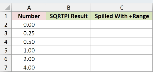
We want to multiply each input by pi and take the square root of that product.
Enter this formula in B2, then copy it down through B7:
=SQRTPI(A2)
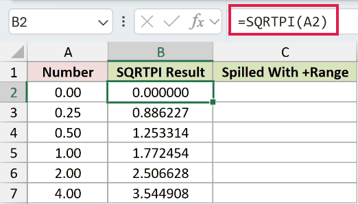
For the input 1.00, the result is 1.772454. The input 4.00 returns 3.544908, while 0.25 returns 0.886227.
Now enter the spilling comparison formula in C2:
=SQRTPI(+A2:A7)
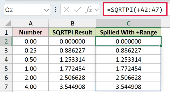
The comparison column displays the same results as column B, but its formula fills C2:C7 automatically. You don’t copy it down.
The leading + turns the range into an array SQRTPI can process. Passing a bare range directly returns a single #VALUE! error.
This spill works in Excel 2021, Excel 2024, and Microsoft 365. In Excel 2019 and earlier, use the per-row formula in column B and copy it down.
Example 2: Calculate a Bell-Curve Height
SQRTPI can also supply the square-root constant inside a longer calculation.
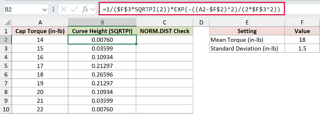
Below is the dataset. Column A lists cap torque, B will hold curve heights, and C will hold comparison results. The setting card contains the mean and standard deviation.
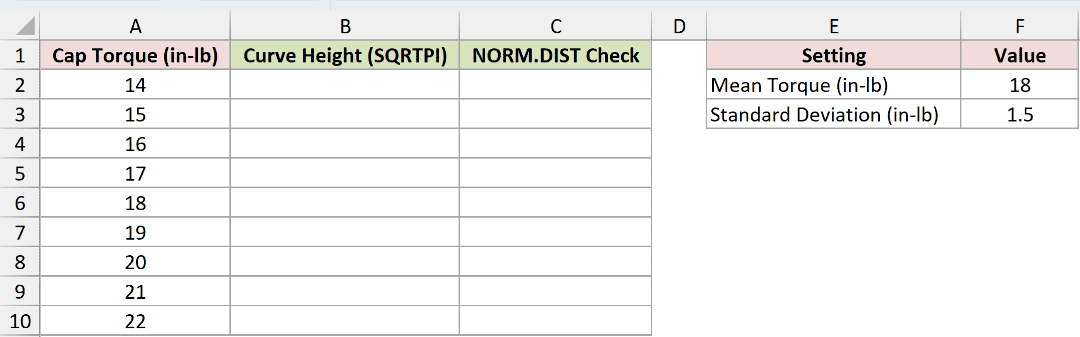
We want the normal bell-curve height at each torque value using the settings in F2:F3.
The mean in F2 is 18 in-lb, and the standard deviation in F3 is 1.5 in-lb. Both settings are typed inputs.
The formula uses EXP, which raises the mathematical constant e to a power, to make the curve fall away from its center.
Enter this formula in B2, then copy it down through B10:
=1/($F$3*SQRTPI(2))*EXP(-((A2-$F$2)^2)/(2*$F$3^2))
How this formula works:
- SQRTPI supplies the square root of twice pi, which is part of the normal curve’s scaling constant.
$F$3supplies the standard deviation, and$F$2supplies the mean. The dollar signs keep both references fixed when you copy down.- The EXP portion uses the squared distance from the mean to reduce the height as torque moves away from the center.
- The parentheses keep the minus sign outside the squared difference.
At torque 18, the curve height is 0.26596. The neighboring inputs 17 and 19 both return 0.21297, showing the curve’s symmetry.
For comparison, NORM.DIST calculates the normal distribution directly. Its FALSE setting returns curve height, so it can check the longer SQRTPI formula.
Enter this comparison formula in C2, then copy it down through C10:
=NORM.DIST(A2,$F$2,$F$3,FALSE)
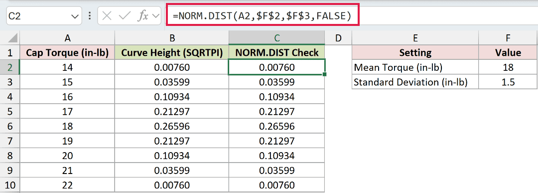
The comparison column matches the displayed SQRTPI-based heights throughout the table, including 0.00760 at torque 14 and 22.
These are curve heights, not percentages or probabilities of an exact torque. SQRTPI supplies a constant here. It doesn’t calculate the standard deviation.
Pro Tip: Use NORM.DIST for routine normal-curve calculations. The expanded SQRTPI formula is useful when you want to see or explain the calculation behind the curve.
Example 3: Calculate Crack Stress Intensity
Here the value inside the square root comes from a measurement on each row.
Below is the dataset. Columns A:C contain part IDs, crack lengths, and applied stresses. Columns D:E will hold intensity and status. The setting card supplies geometry and toughness inputs.

We want to calculate each part’s stress intensity, then compare it with the toughness threshold supplied for this example.
The geometry factor in H2 is 1.12, and the toughness threshold in H3 is 26 MPa√m. Both are typed settings.
Enter this formula in D2, then copy it down through D8:
=$H$2*C2*SQRTPI(B2/1000)
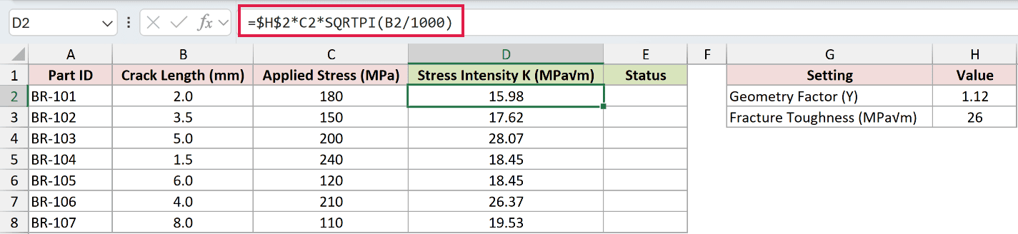
The division inside SQRTPI converts the crack length from millimeters to meters. SQRTPI then takes the square root of pi multiplied by that converted length.
The formula multiplies this term by the applied stress in C2 and the fixed geometry factor in $H$2.
BR-101 returns 15.98 MPa√m, while BR-103 returns 28.07 MPa√m. The different crack lengths and stresses both affect the result.
Next, IF tests a condition and returns the corresponding label. Here it compares the calculated intensity with the threshold.
Enter this formula in E2, then copy it down through E8:
=IF(D2>=$H$3,"Replace","OK")
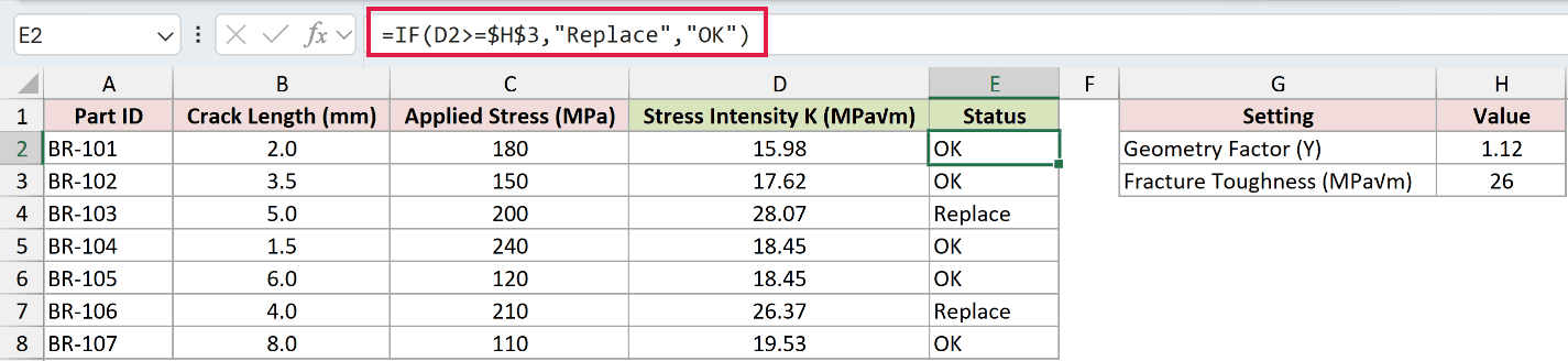
The comparison labels BR-103 and BR-106 Replace, with intensities of 28.07 and 26.37. BR-101 is labeled OK.
The test includes equality, so a result at the supplied threshold also receives Replace.
Example 4: Check Errors and Input Types
Let’s finish by checking inputs that don’t behave like ordinary positive numbers.
Below is the dataset. Column A names each input case, B contains the test inputs, C will hold SQRTPI results, and D provides a manual-calculation comparison.
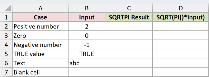
We want to see which inputs SQRTPI accepts and where the manual comparison behaves differently.
Enter this formula in C2, then copy it down through C7:
=SQRTPI(B2)
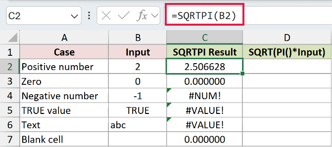
The error rows are deliberate demonstrations:
- The negative input in
B4produces#NUM!inC4because its product with pi is negative. - The TRUE input in
B5produces#VALUE!inC5. SQRTPI doesn’t accept this logical value directly. - The text
abcinB6produces#VALUE!inC6because it cannot be read as a number.
The zero input and the genuinely blank cell both display 0.000000. That blank result is easy to overlook when an input is missing.
For the manual comparison, PI returns the constant pi and SQRT takes a square root. Multiplying the input by pi first reproduces SQRTPI’s calculation for numeric inputs.
Enter this comparison formula in D2, then copy it down through D7:
=SQRT(PI()*B2)
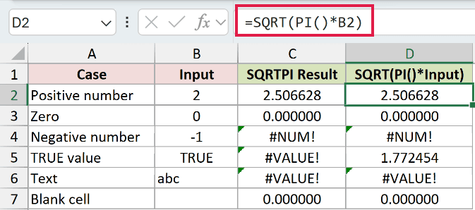
For the positive input, the comparison displays 2.506628, matching SQRTPI. Its negative and text cases deliberately reproduce #NUM! and #VALUE!.
The TRUE row is different: the manual comparison returns 1.772454 because multiplication converts TRUE to a number. SQRTPI’s direct reference returns #VALUE! instead.
Check the intended input type before choosing how to handle it.
Tips & Common Mistakes
- SQRTPI multiplies by pi before taking the square root. It doesn’t divide by pi, so check which operation your mathematical formula needs.
- A bare range produces
#VALUE!. Use the leading-plus form shown in Example 1 when you want a spilled result column. - A blank input is treated as zero. Check missing measurements before interpreting a zero result as a completed calculation.
- Negative inputs produce
#NUM!. Correct the source input when a negative measurement isn’t meaningful rather than hiding the error. - Text that represents a number can be converted, but other text produces
#VALUE!. TRUE also fails when passed directly, as Example 4 demonstrates.
Related Excel Functions / Articles:
