How to Remove Scientific Notation in Excel

While Excel is built to work with large numbers, when you enter a number that has more than 11 digits, you would notice that these are converted into scientific notation (such as 1.234E+11).

This can be perplexing for new Excel users who have no idea why this happens and how to get rid of the scientific notation and get the regular number back.

In this tutorial, I will show you some simple methods you can use to quickly remove the scientific notation and get the original number in the cell.

What is Scientific Notation in Excel?

Scientific notation is a mechanism for representing large numbers in a simplified form. Microsoft Excel is used across various industries that’s why it supports numbers to be stored in scientific format.

In Excel when a number is greater than 11 digits, it’s automatically stored in the scientific notation by replacing part of the number with E+n, in which E (exponent) multiplies the preceding number by 10 to the power n.

For example, the number 4645763434523, which is in standard notation, can be written in scientific notation with 2 decimal places as 4.65E+12. Likewise, we can store negative numbers in scientific notation as well. 

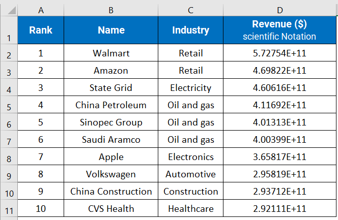
In this tutorial, I am going to use a sample data set that shows the Revenue generated by the top 10 companies in the world. The data is collected from Wikipedia so might not be exact.

Since the revenue figures are large numbers, Excel has converted these into scientific notation.

Now let’s see some methods to get rid of the scientific notation and convert it into a standard notation.

Also read: How to Write Scientific Notation in Excel?

Remove Scientific Notation by Changing the Format of the Cells

By default, the cells in Excel are in the ‘General’ format, which automatically converts numbers that are longer than 11 digits into scientific notations.

And the easiest way to get rid of these scientific notations and get the numbers back would be to change the format of these cells (and apply the Number format).

There are two ways you can quickly change the format of the cells in Excel – using the format cells dialog box, and by using the formatting dropdown in the ribbon.

Using the Format Cells Dialog Box Option

1. Select the range of cells from which you want to remove the scientific notation. In this example, I am going to select the cells in the Revenue column.

2. Click on the ‘Home’ tab in the ribbon

3. Then click on the Format option

4. In the options that show up in the drop-down, click on ‘Format Cells’

5. A dialog box will get open. Select ‘Number’ in the Category options, and change the ‘Decimal places’ value to 0 (unless you want to show decimals in your numbers). After that hit OK.

Once you’re done with the above steps, you will get the Revenue column numbers in standard notation (as shown in the below screenshot).

Bonus tip: There are two more ways to open the Format Cells dialog box in Excel: 

1. Keyboard Shortcut to open Format Cells option – Select the cell and use the keyboard shortcut – CTRL + 1 (hold the CNTRL key and then hit the 1 key)

2. Right-click on the range selected in step 1, and in the options that show up, click on the Format Cells option

Using the Formatting Option in the Ribbon

Another quick way to change the formatting of the cells is by using the formatting drop-down that shows some of the frequently used options.

Below are the steps to change the formatting of the cells to remove the scientific notation and get regular digits back: 

1. Highlight the range from where you want to remove the scientific notation

2. Click on the Home tab in the ribbon

3. In the Home tab, click on the Number Format option.

4. From the drop-down select ‘Number’

The above steps will convert the scientific notation to Number Format (as shown below).

But here you can see that the numbers are in decimal form.

If you don’t want the decimals in the results, you can quickly remove them by following the below steps.

1. Select the range of cells from which you want to remove the decimals

2. Click on the Home tab in the ribbon

3. In the Home tab, there is an option Decrease Decimal. By clicking Once on the option it will remove one decimal digit from the range. In this example we want to remove 2 decimals so click twice.

4. Now the data is in standard notation as shown in the below figure.

In the above section, I have provided a detailed step-by-step explanation of how you can get rid of a scientific notation by using the Format Cells option.

And now, I will show you some other approaches to remove the scientific notation.

Remove Scientific Notation using Excel Formulas

There are various built-in formulas available in Excel using which we can get rid of scientific notation and get our data in standard form.

For this section, I am going to use the following dataset where there are two Revenue columns one shows data in scientific notation, and in the next column, we will convert data to Standard notation by applying different formulas.

Using the TRIM() function

The TRIM function is basically used to remove extra spaces from the text but we can use it to convert Numbers from scientific notation to standard notation as well.

Let’s apply a TRIM function to our data

Hit enter and drag the formula to all the cells. You get the output in standard notation as shown below.

The reason this works is that the output of the TRIM formula is considered as text by Excel.

And since text values are not changed and are shown as is, the result of the TRIM function (which is the entire number) is shown as is without changing it to the scientific notation.

And don’t worry, you can use the result of the trim function as a number in calculations.

Using the CONCATENATE() Function

CONCATENATE function is usually used to join different text values but employing this we can also remove scientific notation in Excel.

Below is the implementation of CONCATENATE function.

Hit enter and drag the formula to all the cells. You get the output in standard notation

Using the UPPER(), LOWER() or PROPER() Function

You can also use any of the above formulas to remove scientific notation. Let’s see them one by one.

In general, the UPPER() function is used to convert text to uppercase, but could be utilized to remove scientific Notation.

Here is the syntax of the UPPER() function.

Similarly, you can use the LOWER or the PROPER formula to convert numbers to scientific notation.

While these functions aren’t made to work with text data, since we’re using them with numbers, they do nothing in return the output as is.

And since the output is now considered as a text value, Excel does not change the number to scientific notation and gives us the number in the original format.

Remove Scientific Notation by converting Number to Text

If you can somehow convert the number into a text value, Excel would leave it alone and would not try and change its format.

This solution should work in most cases, even if you plan to use the output in formulas (as most formulas are built to convert text values to numbers in such scenarios). However, there would be some formulas that could consider the result of the methods I will show in this section as text values, and would ignore them (such as the SUM function or the AVERAGE function).

By Adding an Apostrophe (‘) Before the Number

While entering data into the cell, if you want to always input data in standard notation, place the apostrophe sign before the number.

This will store the number in text format and prevent it from getting converted into scientific notation.

Below I have a data set where I have the revenue of the top ten companies in the world. and as you can see, the revenue figures have been changed into scientific notation by Excel.

Below are the steps to add an apostrophe before the number remove the scientific notation:

1. Select the cell from which you want to remove the scientific notation

2. Double-click on the cell to Edit it or press F2 from the keyboard.

3. Place an apostrophe sign at the beginning of the Number

4. This will convert the Number to standard notation.

While this method works, the drawback of this method is that you will have to manually go and add the apostrophe for each number.

This could be useful in case you are manually entering the data, where you can add the apostrophe while you’re entering the data.

But in case you already have the data in the scientific notation, it may be a bit cumbersome to manually add the apostrophe before each number.

In such a case, it would be better to use the formatting method covered earlier or the formula method covered just prior to this method.

Alternatively, you can also use a third-party add-in method covered next.

By using Kutools Add-in

Kutools is a handy Excel Add-in that incorporates more than 300+ features.

It assists you in performing complex tasks swiftly and easily. In addition, using Kutools you can convert Numbers to Text and vice versa effortlessly.

Below are the steps to download and install the Kutoolsa add-in in Excel:

1. Kutools is not a built-in feature in Excel. It is an Excel Add-in that you have to manually install on your computer. Here is the link from where you can download this Add-in free of cost Kutools
2. Download and install the Add-in
3. After installation, it appears in the Ribbon as shown

Now in order to remove scientific notation using Kutools follow the steps

1. Select the range from where you want to remove scientific notation. In this example, I am going to select the Revenue column values.

2. Click on the Kutools option in the ribbon

3. Now from the option click on Content

4. Click on the ‘Convert between Text and Number’ option in the drop-down list

5. Doing so a dialog box gets open. Select the ‘Number to text’ option and hit OK.

6. This will remove the scientific notation from the selected range by converting the Number to Text. The result is shown in the screenshot.

By Changing the Column Width

Another scenario where Excel may convert your numbers into scientific notations is when the column width is less and cannot accommodate the entire number.

Instead of showing you a truncated number, Excel converts the number into scientific notation that can fit within the column width.

And this can happen even if you have less than 11 digits. For example, below I have a number 123456789 in cell A1, but since the column width is less, you see the scientific notation instead.

If this is not something you want, this has an easy fix – increase the column width.

And there are multiple ways to do it:

• Double-click on the right edge of the column header (the one that contains the column alphabet). This would expand the column to fit the content of the cells

• Place the cursor on the edge of the column header, right-click and drag to expand the column width

• Right-click on the column header, and then click on column width. This would open a dialog box where you can specify the column width manually.

In this tutorial, I covered multiple ways you can use to get rid of scientific notation in Excel. The easiest way would be to change the formatting of the cells so that the numbers are shown with all the digits instead of the scientific notation.

You can also use text formulas such as TRIM or UPPER/LOWER/PROPER to quickly convert the numbers in scientific notation into text values that are shown with all the digits in the number.

And in the case of Excel converting numbers into scientific notation because the column width is low, you can easily fix this by increasing the column width.

Other Excel articles you may also like:

• How to Convert Decimal to Binary in Excel
• How to Remove Space before Text in Excel (5 Easy Tricks)
• How to Extract Numbers from Text in Excel (Beginning, End, or Middle)
• How to Remove Text after a Specific Character in Excel (3 Easy Methods)
• How to Convert Radians to Degrees in Excel (Easy Formula)
• How to Apply Accounting Number Format in Excel