Excel by default displays negative numbers with a minus sign.
In some instances, for example, when dealing with financial data, you may want to display negative numbers in parentheses or brackets for better readability.
In this tutorial, I am going to show you two easy ways to show negative numbers in parentheses/brackets in Excel.
Method #1: Use Excel’s Built-in Number Format
The following is a dataset that shows the annual incomes of three families in the years 2019 and 2020. The increase or decrease of the incomes is shown in column D. I want the negative values displayed in parentheses.

Excel has a built-in number format for displaying negative numbers in parentheses.
Note: Number formats only change how numeric data is displayed in cells. They do not alter the underlying numbers that are stored in the cells.
We use the steps below to apply the built-in number format:
- Select range D2:D4.

- Open the Format Cells dialog box by using any of the following ways:
Press Ctrl + 1
Or
Right-click the selected range and choose Format Cells on the shortcut menu:

Or
Select the Home tab, and click the Number Format dialog box launcher icon in the right bottom corner of the Number group:

- In the Format Cells dialog box, check that the Number category is selected in the Category list box. In the Negative numbers list box on the right select the option that displays a negative number in parentheses in black color and click OK.

The negative numbers in column D are now displayed in parentheses:

Also read: How to Apply Accounting Number Format in Excel
What to do if you don’t see the negative numbers in parentheses built-in format
Sometimes you may not see the built-in option for displaying negative numbers in parentheses listed in the Negative numbers list box of the Format Cells dialog box.
Do the following steps to have the option displayed:
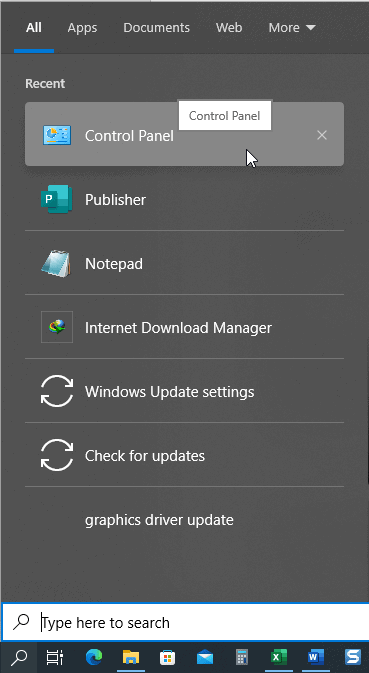
- Open the Control Panel app in Windows.
- Choose the Clock and Region option in the Control Panel window.

- In the Clock and Region window, choose the Region option.

- In the Region dialog box that appears, in the Formats tab, click the Additional Settings button.

- In the Customize Format dialog box, in the Numbers tab, in the Negative number format drop-down list, select the option that shows a number displayed in parentheses, and click Apply then OK.

- In the Region dialog box, in the Formats tab, click Apply, then click OK.

You should now have the option for the display of negative numbers in parentheses listed in the Negative numbers list box in the Format Cells dialog box in Excel.

Also read: Format Numbers to Show in Millions in Excel
Method #2: Use a Custom Number Format
The built-in number format for displaying negative numbers in Excel has only two default display options.
The first option shows negative numbers in parentheses in black color and the second option shows negative numbers in parentheses in red color.

Sometimes you may want to display negative numbers in parentheses but in other ways other than the two default options.
For instance, you may want the negative numbers displayed in parentheses but in blue color, or the negative numbers displayed in parentheses preceded with a minus sign, and so on.
To achieve this you must first build a custom number format.
For a better understanding of how to build a custom number format in Excel, we first explain the components of a custom number format in Excel.
Understanding Custom Number Format in Excel
A cell in Excel can contain any of the following types of data:
- A Positive number
- A Negative number
- A Zero value
- Text
When building a custom number format you have to specify how each of the above data is to be displayed in a cell.
A custom number format can have up to four sections separated by semicolons. The structure is as follows:
<Format for Positive Number>;<Format for Negative Number>;<Format for Zero>;<Format for Text>
Points to remember:
- Although the custom number format can have up to four sections, only one section is required. If you want to skip a section, type a semi-colon in the proper place without specifying a number format code.
- The General format is assumed in case you do not specify the format code for any of the four types of data.
- When only one number format is specified, Excel uses that format for all types of data.
- If you create a custom number format that has only two sections, the first section is used for positive values and zeros and the second section is used for negative values. The General format is used for text values.
When building custom number formats, we use the following characters as placeholders:
- Zero (0) This character is used as a placeholder for insignificant zeros.
- Pound sign (#) This character is a placeholder for significant digits.
- Question mark (?) It is used to show aligned decimals.
- Period (.) This is used as a placeholder for a decimal point in a number.
- Comma (,) This is used as a placeholder for the thousands separator.
- Asterisk (*) This is used to force characters to repeat.
- Underscore (_) This is used to add space in a number format.
- At (@) This is a placeholder for text.
Excel supports the following eight colors in custom number formats. The color names must be entered in square parentheses as shown below:
- [Black]
- [White]
- [Red]
- [Green]
- [Blue]
- [Yellow]
- [Magenta]
- [Cyan]
With that information out of the way, let’s now build a custom number format to display negative numbers in column D in parentheses and in blue color:

We use the following steps:
- Select range D2:D4.

- Open the Format Cells dialog box by using any of the following ways:
Press Ctrl + 1
Or
Right-click the selected range and choose Format Cells on the shortcut menu:

Or
Select the Home tab, and click the Number Format dialog box launcher icon in the left bottom corner of the Number group:

- In the Format Cells dialog box, in the Number tab, select the Custom category in the Category list box.

- Replace the number format that is in the Type text box on the right with the following custom number format and click OK:
#,##0.00;[Blue](#,##0.00)

The negative values in column D are now displayed in parentheses/brackets in blue color.

This tutorial showed you how to change the number format of cells so that negative numbers are displayed in parentheses.
It also showed you how to build a custom number format to display negative numbers in parentheses and in another color other than Excel’s default red color.
Of the two methods, while the in-built custom format method is fast, the second method (using custom format code) allows you a lot more control. For example, you can choose to show negative numbers in parentheses while also keeping the minus sign, or show negative numbers in brackets and in a color other than red.
Other articles you may also like:
- How to Count Negative Numbers in Excel – Easy Formula
- How to Make Positive Numbers Negative in Excel
- How to Change Font Color Based on Cell Value in Excel?
- How to Remove Table Formatting in Excel?
- Remove Parentheses (Brackets) in Excel
- Remove Negative Sign in Excel
- How to Format Phone Numbers in Excel
- How to Add Zero In Front of Number in Excel (7 Easy Ways)