Format Numbers to Show in Millions in Excel

Formatting large numbers in millions in Excel makes the numbers easier to read and understand.

Formatting numbers in millions makes the data more concise and avoids cluttering the worksheet with unnecessary digits making it easier for readers to compare and interpret data. 

In this article, I will show you four techniques for formatting numbers in millions in Excel.

Method #1: Apply a Custom Number Format to Format Numbers in Millions in Excel

We can use custom number formatting to format numbers in millions in Excel.

Let’s consider the below-shown dataset showing the population of some of the most populous states in the USA.

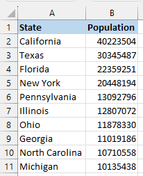
The population numbers are in a general format, meaning they do not have a specific number format. 

While the numbers are alright, it would be helpful to show these figures in millions (as it would make it easy to comprehend and compare the figures)

To format the population of the states in millions, use the following steps:

1. Select the cell range B2:B11 containing the population figures.

2. Right-click the selection and click the Format Cells option on the context menu to open the Format Cells dialog box. Alternatively, you can press the shortcut Ctrl + 1.

3. On the Format Cells dialog box, open the Number tab, select the Custom category on the left, and replace whatever is on the Type box on the right with the following number format code:

0,, “Million” 

4. Click OK.

The population figures are now formatted in millions:

Note: Formatting numbers in millions in Excel using a custom number format does not change their value. Formatting changes the way that the numbers are displayed on the screen, but it does not alter the underlying values of the cells, as seen below:

Explanation of the Number Format Code

0,, “Million” 

The zero instructs Excel to display the number exactly as it appears in the cell.

The first comma tells Excel to cut off the number’s last three digits, and the second comma instructs Excel to cut off the next three digits. So, the two commas remove six digits from the number. 

And, of course, the “Million” adds the suffix “Million” to the remaining digits. 

Note: If you want the numbers formatted with one decimal place and an “M” suffix, enter the following number format code on the Type box:

0.0,, "M"

The numbers will be displayed as shown below:

Also read: Excel Showing Formula Instead Of Result

Method #2: Use the TEXT Function to Format Numbers in Millions in Excel

We can use the TEXT function to format numbers in millions in Excel.

However, the result will be text strings and not numeric values and, therefore, cannot be used in numeric calculations. 

Let’s look at the following dataset showing the population of the ten most populous states in the USA.

The population figures are in a general format, meaning they are not in a specific number format. 

We want to apply the TEXT function to format the population numbers in column B in millions and display them in column C.

Below are the steps to get this done in Excel:

1. Select cell C2 and enter the below formula:

=TEXT(B2,"0,, ")&"Million"

2. Copy the formula down the column by double-clicking or dragging the fill handle feature.

Notice that the resultant values in column C are left-aligned, meaning they are text strings and cannot be used in numeric calculations.

Explanation of the formula

=TEXT(B2,”0,, “)&”Million”

In this formula, the TEXT function uses the “0,, ” format code as the format_text argument to remove six digits from the value in cell B2 and add space.

The ampersand operator (&) is then used to join the suffix “Million” to the value returned by the TEXT function.

Note: To format the numbers with one decimal place and append an “M” suffix, use the below-given formula:

=TEXT(B2,"0.0,, ")&"M"

The numbers will be displayed as follows:

Note: When you use the TEXT function to matt numeric values, the result that you get is a text string. This means that you cannot use the result of the text function in numeric calculations. But on the plus side, you can easily send any text at the beginning or the end of the result of the text function. For example, in our example, I can use the following formula to show the state name along with the population invariants as the result of the text function =A2&” – “&TEXT(B2,”0.0,, “)&”M”

Method #3: Use the ROUNDUP Function to Format Numbers in Millions in Excel

You can use a formula with the ROUNDUP function to format numbers in millions in Excel. 

Suppose we have the below-shown dataset showing the population of the ten most populous states in the USA.

The population figures are in a general format, meaning they are not in a specific number format. 

We want to apply the ROUNDUP function in a formula to format the population numbers in column B in millions and display them in column C.

We proceed as follows:

1. Select cell C2 and enter the formula below:

=ROUNDUP(B2/10^6,0)&" Million"

2. Copy the formula down the column by double-clicking or dragging the fill handle feature.

Note that the values we get in column C are aligned to the left of the cell.

This indicates that these are text strings, and we cannot use these in numeric calculations.

Note: In case you want the result of the ROUNDUP function to be numeric values that can be used in further calculations, do not append any text before or after the result of the ROUNDUP function

Explanation of the formula

=ROUNDUP(B2/10^6,0)&” Million”

The value in cell B2 is divided by a million (10^6). Then, the ROUNDUP function uses the zero (0) num_digits argument to round up the quotient to the nearest integer.

Finally, we use the ampersand operator (&) to join the “Million” suffix with a leading space to the integer.

Note: Use the below formula if you want to format the numbers with one decimal place and append an “M” suffix:

=ROUNDUP(B2/10^6,1)&" M"

The population figures in millions will be displayed in column C as follows:

Also read: How to Round Numbers in Excel Without Formula?

Method #4: Change Display Units on the Format Task Pane to Display Millions on a Chart

Suppose you want to create a chart based on the dataset below that has the population of ten states in the USA.

You want to create a bar chart based on the dataset and display the population in millions.

Here’s how you do it:

1. Select the entire dataset.
2. On the Insert tab, click Recommended Charts on the Charts group.

3. Select the Clustered Column chart on the Insert Chart dialog box and click OK.

4. Right-click the y-axis on the chart and select Format Axis on the context menu to open the Format Axis task pane on the right of the Excel window.

5. On the Format Axis task pane, open the Display units drop-down and choose Millions.

The population is now displayed in millions on the graph.

Also read: How to Switch Axis in Excel (Switch X and Y Axis)

This tutorial showed four techniques for formatting numbers in millions in Excel.

The first technique involves using custom number formatting; the second applies the TEXT function in a formula; the third uses a formula involving the ROUNDUP function; and the fourth method applies to changing the display units on a graph. 

We hope you found the tutorial helpful.

Other Excel articles you may also like:

• Show Formulas (Instead of Formula Result) in Excel (Shortcut)
• Show Negative Numbers in Parentheses/Brackets in Excel
• How to Write Scientific Notation in Excel?
• Apply Comma Style Number Format in Excel
• Data Types in Excel
• How to Apply Accounting Number Format in Excel