While Excel is designed primarily for calculations and data analysis, you can also insert images into cells.
This feature proves valuable when creating product catalogs, inventory lists, or employee directories. For instance, if you’re creating product catalogs, you may want to have the product names in one column and their images in another column.
I will show you ways to insert an image in a cell in Excel from your device, clipboard, stock images in Microsoft’s built-in image library, or from the web.
Method #1: Paste an Image in a Cell from the Clipboard
The easiest way to insert an image in a cell is to copy it to the clipboard and then paste it into a cell.
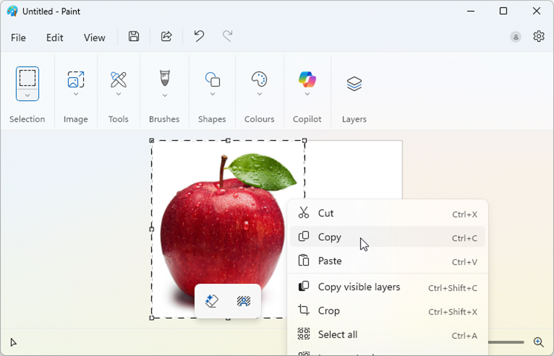
Suppose you have an image in another program, for example, Paint. You can insert it into a cell using the steps below.
- Right-click the image and copy it to the clipboard.
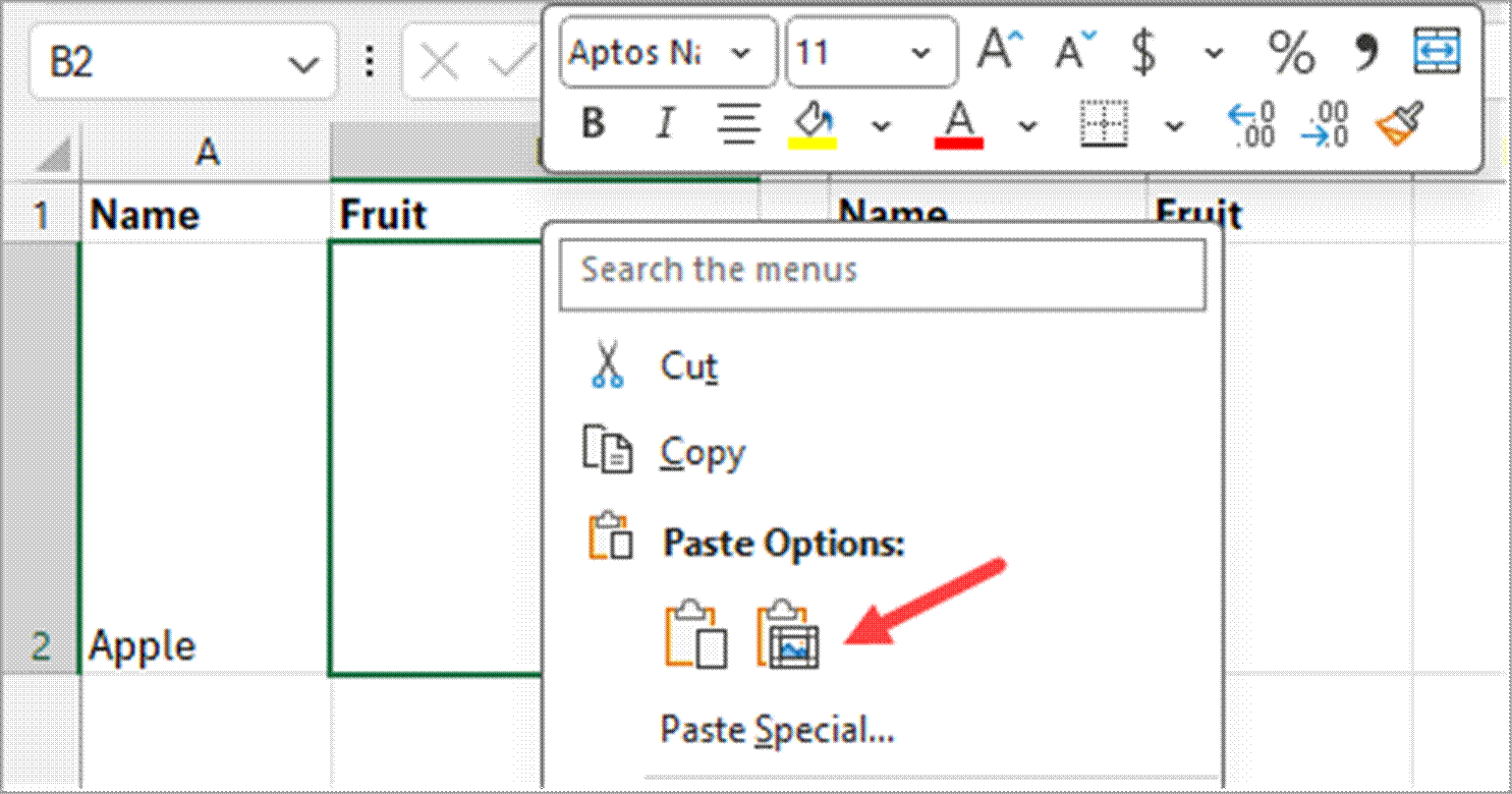
- Right-click the cell where you want to insert the image.
- Under the Paste Options section on the shortcut menu, click the Paste Picture in Cell option.
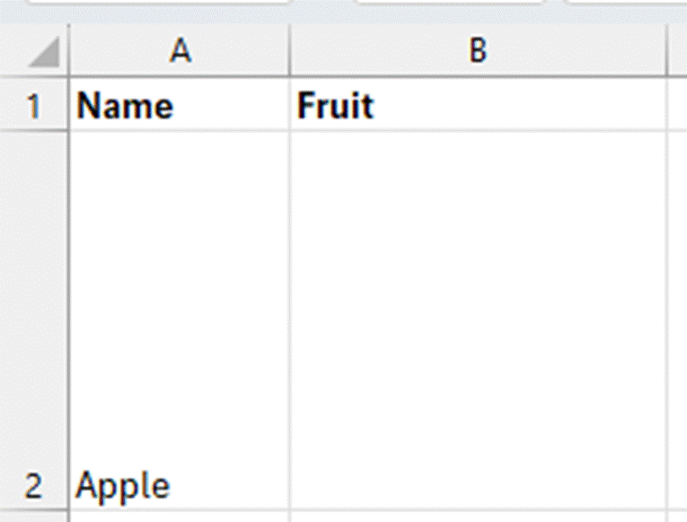
The image you copied to the clipboard is pasted into the target cell.

Note: If you use the CTRL + V or the default paste option on the Ribbon, the picture will be pasted over cells and not into the target cell.
Method #2: Insert an Image in a Cell from the Ribbon
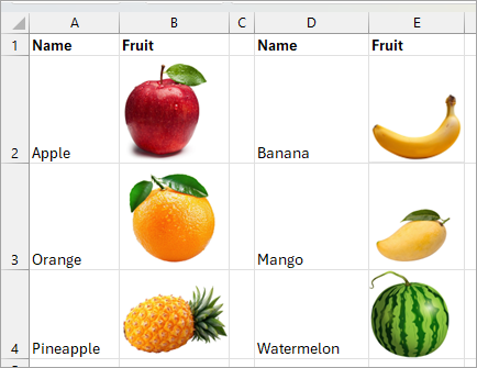
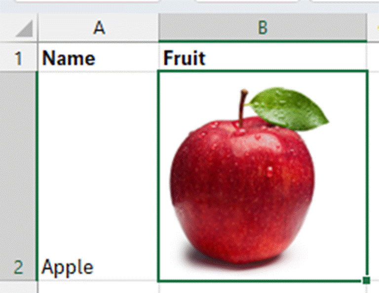
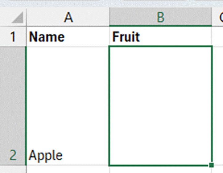
Suppose you want to insert the image of an apple in cell B2 to correspond with the name of the fruit in cell A2.
This is how you can do it from the Ribbon:
- Select cell B2.
- Open the Insert tab.
- On the Illustrations group, open the Pictures drop-down, hover the mouse pointer over the Place in Cell option to open the Insert Picture From submenu.
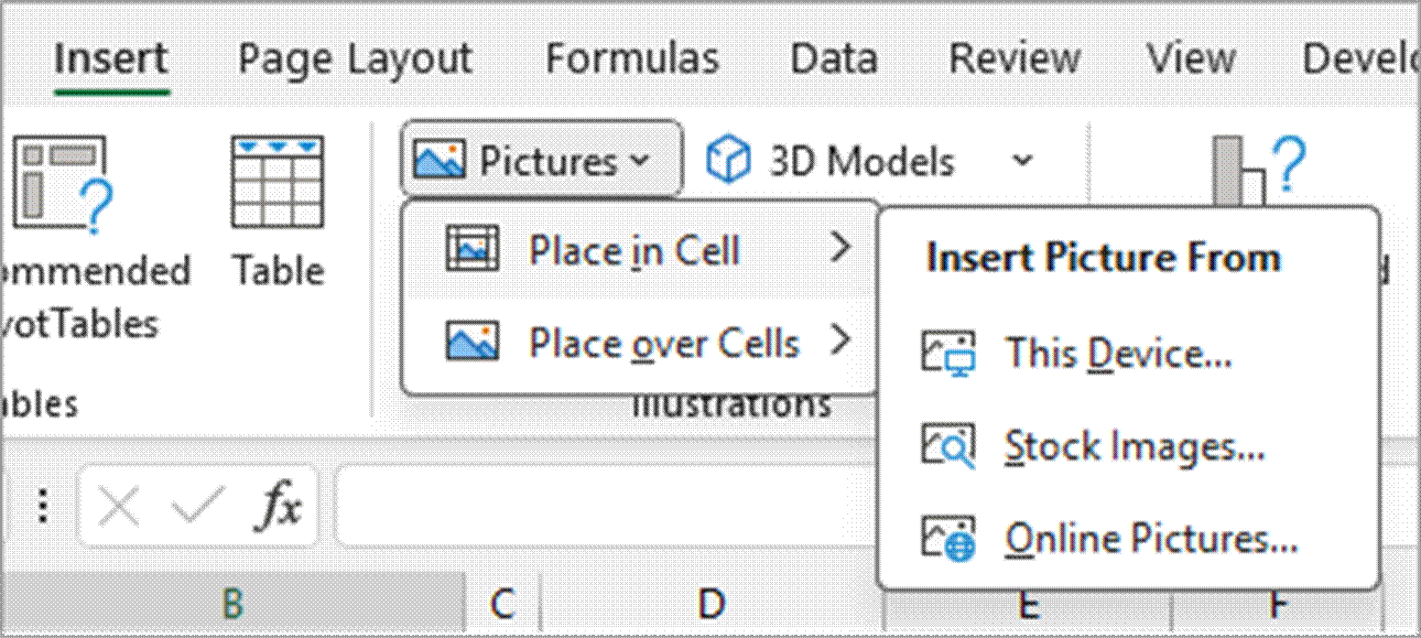
- Select one of the following options from the Insert Picture From submenu:
- This Device – to insert an image stored locally on your device.
- Stock Images – to insert an image from the stock images in Microsoft’s built-in image library.
- Online Pictures – to insert a picture from the web.
In this case, I have selected the “This Device” option to insert an image stored locally on my device.
- Navigate to where the target image is stored, select it, and click Insert.
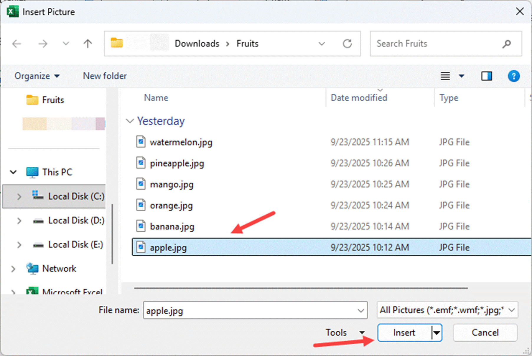
The image you have selected is inserted into cell B2.

How to Insert Multiple Images
To insert multiple images, do the following:
- Navigate to where the images you want to insert are stored, as shown in steps 4 and 5 above.
- Select one image, press the CTRL key as you select the other images in sequence, and click Insert.
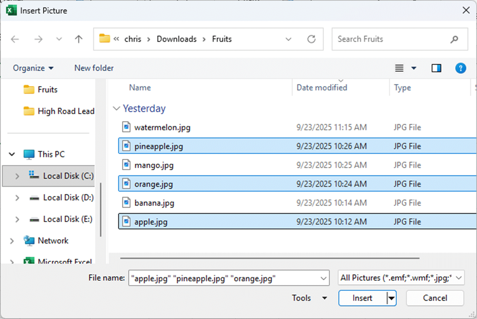
Note: To select all images in the folder, select the first image, press the Shift key, and select the last image.
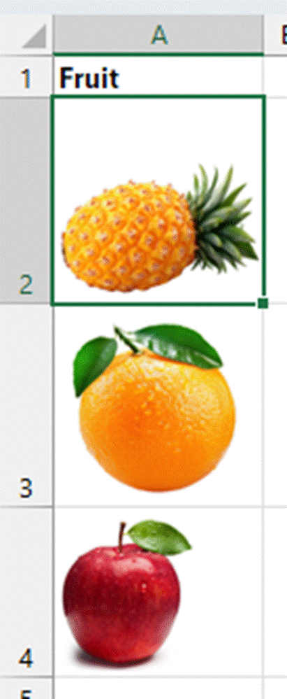
All the images you have selected are inserted into the target cells, starting from the active cell and down the column for as many cells as the images you selected.
Method #3: Switch a Picture Floating Over Cells to a Picture in a Cell
When you use CTRL + V or the default paste option on the Ribbon to paste a picture in Excel, the image is pasted over cells and not into a cell.
You can switch the picture floating over cells to an image in a cell by selecting the picture and clicking the Place in Cell command button at the top right corner of the image.
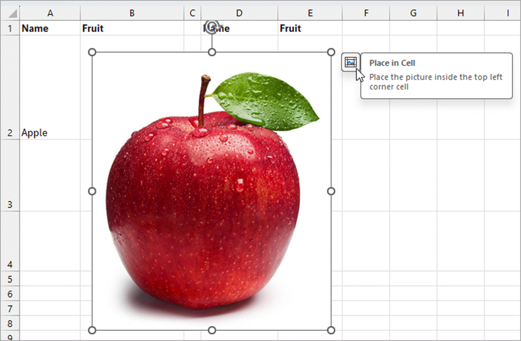
The image is placed inside the cell at the image’s top left corner.
How to Add Alt Text to Images
It is good practice to add alt text (short for alternative text) to the images you insert in your workbooks.
Alt text is a short description of an image. It serves two main purposes:
- Accessibility – Screen readers read alt text aloud so that people who are blind or visually impaired can understand what the image is about.
- Fallback content – If an image doesn’t load (due to a slow connection, broken link, or other issue), the alt text appears in its place so users still get the context.
Example
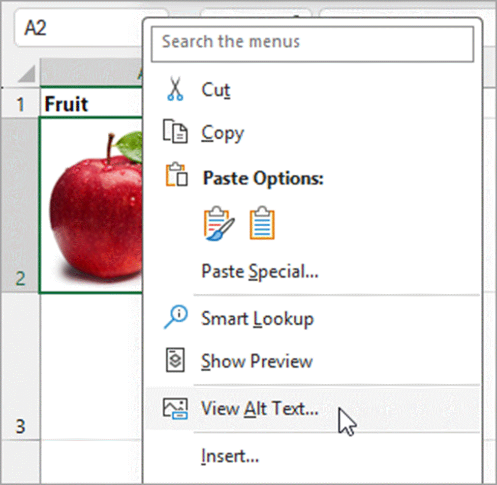
To add alt text to an apple image in cell A2, do the following:
- Right-click the image and choose View Alt Text on the context menu.
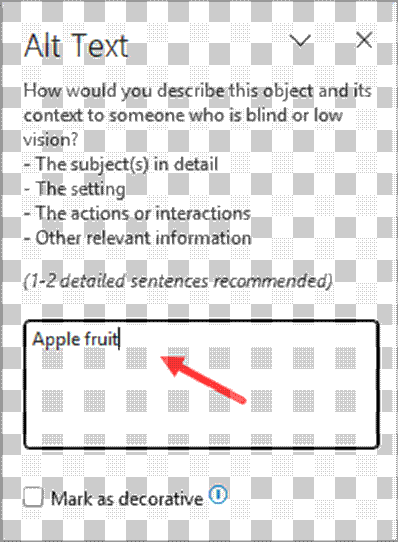
The above step opens the Alt Text task pane on the right of the Excel window.
- Fill the alt text in the task pane.
Method #4: Use the IMAGE Function
The IMAGE function allows you to insert an online image directly into a cell by referencing its URL.
The Syntax of the IMAGE Function:
=IMAGE(source, [alt_text], [sizing], [height], [width])
Only the ‘source’ argument is required. All the others are optional.
- source argument refers to the URL or web link of the image. The image must be publicly accessible (direct link ending with .png, .jpg, etc.).
- alt_text refers to alternative text or description for accessibility. It is useful for screen readers, and if the picture does not load.
- sizing controls how the picture fits into the cell and can be 0 (default, fit image to cell), 1 (fit cell, ignore aspect ratio), 2 (keep original file size, may overflow cell), or 3 (custom size, requires height and width arguments).
- height is used if sizing is custom. It sets the height of the image in pixels.
- width is supplied if sizing is custom. It sets the width of the image in pixels.
Example
Suppose you want to insert into cell B2 an image of an apple whose link is: https://freepngimg.com/thumb/apple_fruit/24454-5-apple-fruit-transparent-image.png
Note: Cell A2 containing the name of the fruit will be used as the alt text argument in the formula.
Here’s how you can do it:
- Copy the URL to another cell, say cell G2. This trick helps you get past the 255-character URL limit.
- Enter the following formula in cell B2:
=IMAGE(G2,A2,0)
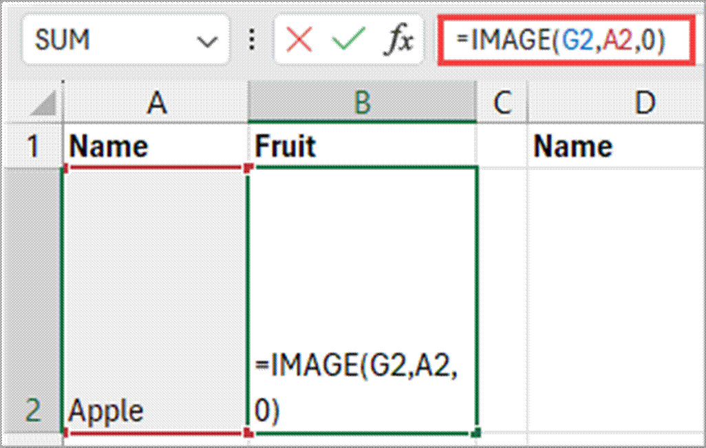
- Press Enter.
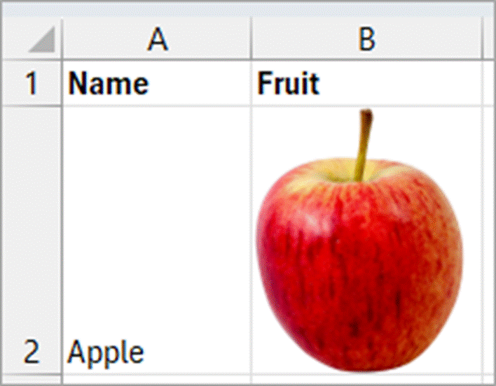
The formula inserts the image of an apple into cell B2, the picture is fitted within the cell, and the alt text is “Apple.”
Note: The fastest way to get the URL of an online image is to right-click it and select “Copy image link” from the shortcut menu.
Notes
- The image won’t display if the source is a URL that is not public (requires authentication).
- If the source URL redirects, Excel blocks it because of security concerns. A redirect occurs when the source URL does not go directly to the target address but to a different one.
I have shown you ways to insert an image in a cell in Excel. I hope you found the tutorial helpful.
Other Excel articles you may also like: