When Excel’s filter stops working, you may find that filter buttons are missing, the criteria don’t apply correctly, or Excel only filters part of your data.
In this tutorial, I explain the reasons Excel filters may stop working and show you how to fix each one.
Reason #1: Dataset Has Empty Columns
An empty column in a dataset can prevent the Excel filter from functioning correctly, as Excel treats it as a break in the data range.
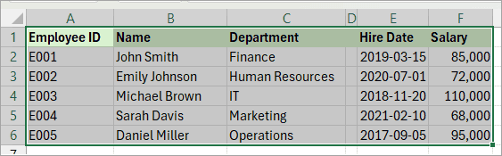
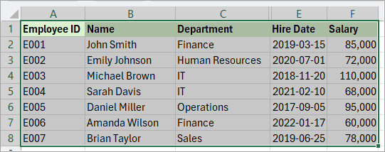
The example dataset below has an empty column D.
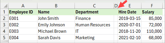
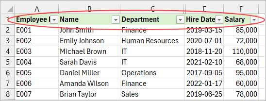
When you turn on filtering, filter buttons will only appear in the first three columns preceding the empty one.
Excel has only applied a filter up to the empty column, ignoring the remaining columns. You will only be able to filter on the columns with the filtering buttons, but not the rest.
Excel expects a continuous range when applying filters. An empty column indicates the end of the data range, so Excel stops recognizing the columns beyond it as part of the same dataset.
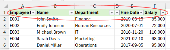
Fix #1: Select Entire Dataset and Apply Filter
- Press CTRL+SHIFT+L to clear the current filter.
- Manually select the entire dataset.
- Press CTRL+SHIFT+L to reapply the filter.
Excel displays filtering buttons in all the columns.
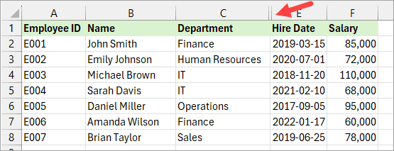
Fix #2: Delete the Empty Column and Reapply the Filter
- Press CTRL+ SHIFT+L to clear the filter.
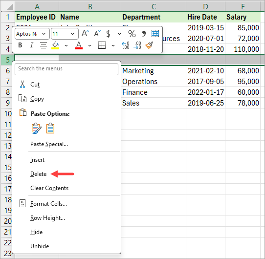
- Delete the empty column by right-clicking its letter header and choosing Delete on the shortcut menu.
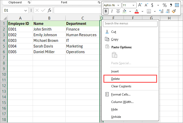
- Select any cell in the dataset and press CTRL+SHIFT+L to reapply the filter.
Excel displays filtering buttons in all the columns of the dataset.
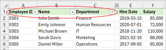
Fix #3: Convert the Dataset to a Table
- Manually select the entire dataset.
- Press CTRL+T to convert the dataset to a table.
You can now use the table’s built-in filtering buttons.
Reason #2: Dataset Has Empty Rows
An empty row breaks a dataset into separate ranges, causing the Excel filter to apply only to a part of the data.
The example dataset below has an empty row 6.
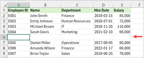
When you enable filtering, Excel applies the filter only to the data range above the empty row.
Fix: Delete the Empty Row and Reapply the Filter
- Press CTRL+ SHIFT+L to clear the filter.
- Delete the empty row by right-clicking its number header and selecting ‘Delete’ from the shortcut menu.
- Press CTRL+SHIFT+L again to reapply the filter.
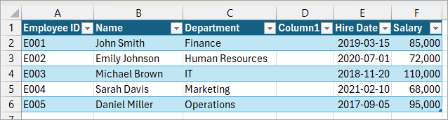
Reason #3: The Dataset Has Empty Hidden Columns
An empty hidden column in a dataset can prevent the Excel filter from functioning correctly, as Excel treats it as a break in the data range.
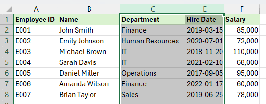
The example dataset below has a hidden empty column D.
When you turn on filtering, Excel only applies a filter up to the hidden empty column, ignoring the remaining columns.
Excel interprets the hidden column as indicating the end of the data range and stops recognizing the columns beyond it as part of the same dataset.
Fix #1: Manually Select the Dataset and Reapply the Filter
- Press CTRL+SHIFT+L to clear the current filter.
- Manually select the entire dataset.
- Press CTRL+SHIFT+L to reapply the filter.
Excel displays filtering buttons in all the columns of the dataset.
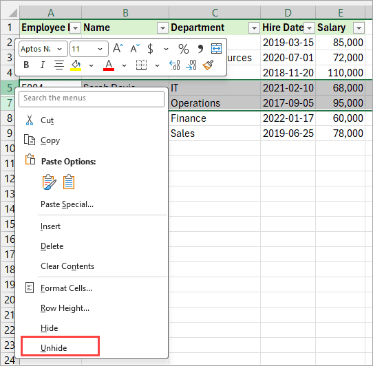
Fix #2: Unhide the Empty Hidden Column, Delete it, and Reapply the Filter
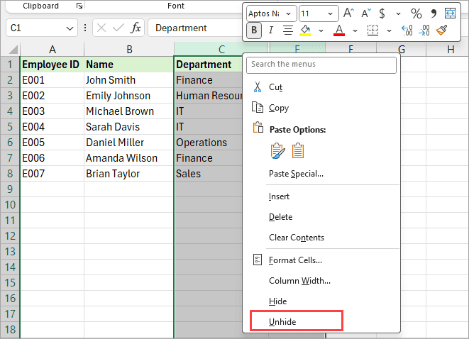
- Select the columns on either side of the hidden empty column by dragging across their letter column headers.
- Right-click the selected column headers and choose Unhide on the shortcut menu.
- Delete the unhidden column as described in Reason #1.
- Press CTRL+SHIFT+L to reapply the filter.
Fix #3: Convert the Dataset to a Table
Select the entire dataset and convert it to a table as described in Reason #1.
Unhide All the Hidden Empty Columns
If your dataset has many hidden empty columns, you can unhide all of them at once using the steps below.
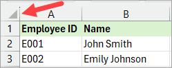
- Click the triangle on top of row 1 and to the left of column A.
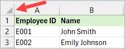
The above step selects the entire worksheet.
- Right-click the selected column letter headers and choose Unhide on the shortcut menu.
Reason #4: The Dataset Has Hidden Empty Rows
An empty hidden row breaks a dataset into separate ranges, causing the Excel filter to apply only to a part of the data.
The example dataset below has an empty hidden row 6.
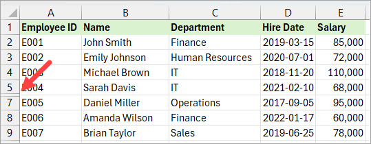
When you enable filtering, Excel applies the filter only to the data range above the empty hidden row.
Fix #1: Manually Select the Entire Dataset and Reapply the Filter
- Press CTRL+SHIFT+L to clear the current filter.
- Manually select the entire dataset as described in the sections above.
- Press CTRL+SHIFT+L to reapply the filter.
Excel applies the filter to the entire dataset.
Fix #2: Unhide the Hidden Empty Row and Delete it
- Select the rows on either side of the hidden row by dragging across their number row headers.
- Right-click the selected row number headers and choose Unhide on the shortcut menu.
- Delete the unhidden row as described in Reason #1.
- Press CTRL+SHIFT+L to reapply the filter.
Unhide All the Empty Hidden Rows
If your dataset has many empty hidden rows, you can unhide all of them at once using the steps below.
- Click the triangle on top of row 1 and to the left of column A.
The above step selects the entire worksheet.
Right-click the selected row number headers and choose Unhide on the shortcut menu.
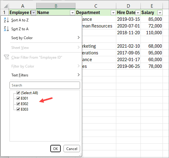
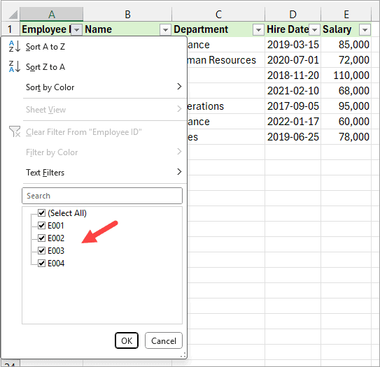
Reason #5: Dataset Column Contains an Error Value
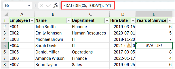
The example dataset below has an error value in cell E5.
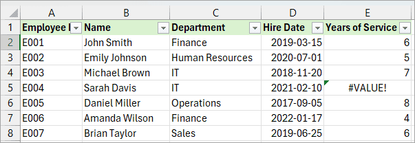
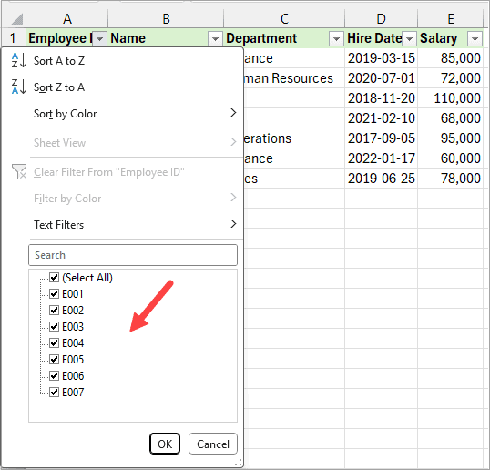
When you try to apply a number filter to column E, let’s say ‘Above Average’, nothing happens.
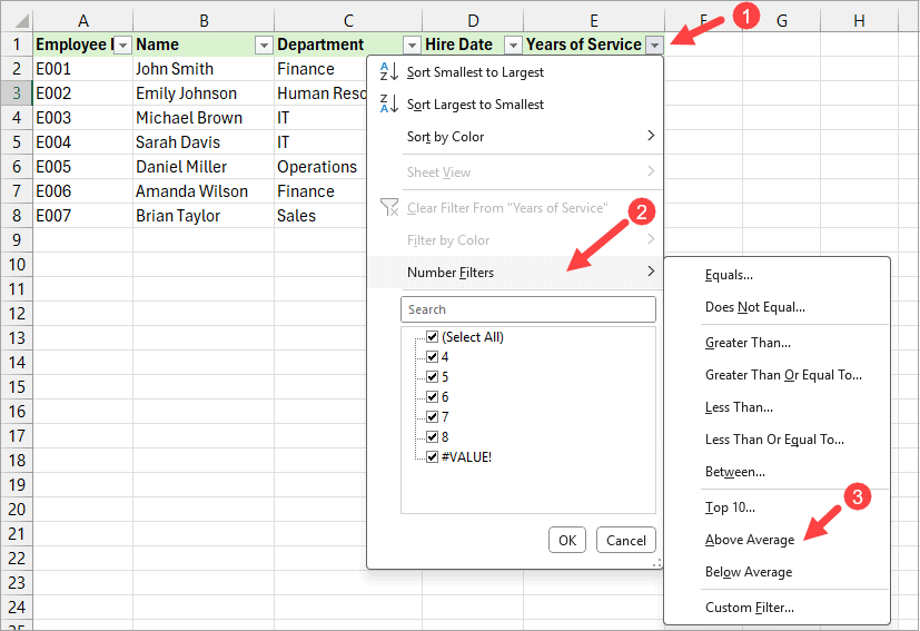
Nothing happens because of the error value in cell E5.
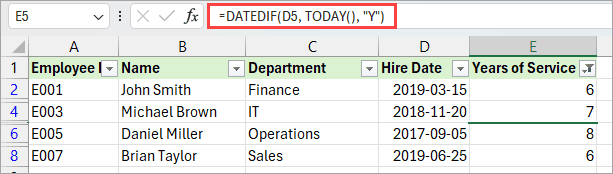
Fix: Resolve What is Causing the Error Value
When you examine the formula in cell E5 of the example dataset, you’ll notice that it references the text value in cell C5 rather than the date value in cell D5.
Once you correct the formula, the error value disappears, and the number filter (‘Above Average’ in this case) works as expected.
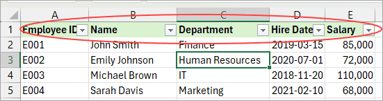
Reason #6: Dataset Column Has Inconsistent Formatting
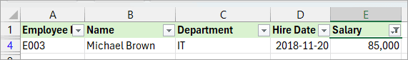
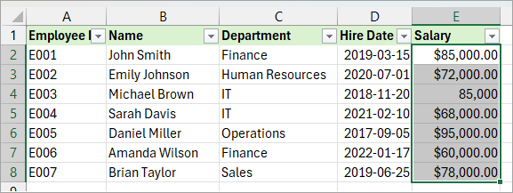
The example dataset below has inconsistent currency formatting in column E.
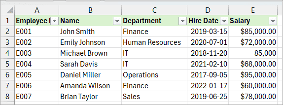
Notice that the employees in rows 2 and 4 each earn $85,000. However, the salary in row 2 is formatted as Currency, while the value in row 4 is formatted as Number.
When, for example, you apply an ‘equals 85,000’ number filter on column E…
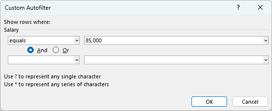
You get only one record instead of the expected two.
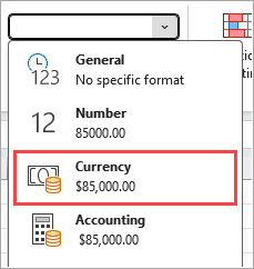
Fix: Apply Consistent Formatting in Column
- Select all the data in the target column.
- Click the Home tab.
- Open the Number Format drop-down on the Number group and choose the relevant formatting (Currency in this case).
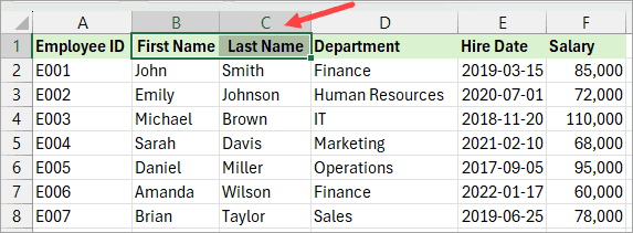
Reason #7: Dataset Has Merged Cells in the Header
Cells B and C in the header of the example dataset below are merged.
If you turn on filtering, the filter in the merged cell will only apply to column B. This is because in a merged range, Excel treats only the left-most cell as containing the value.
Fix: Unmerge the Cells and Enter Separate Column Headings
- Press CTRL+ SHIFT+L to clear the filter.
- Select the merged cells.
- Click the Home tab.
- On the Alignment group, open the Merge & Center drop-down and choose Unmerge Cells.
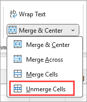
The above step unmerges the merged cells.
- Enter separate column headings in the unmerged cells.
- Press CTRL+SHIFT+L to reapply the filter.
Excel displays filter buttons in each of the unmerged cells.
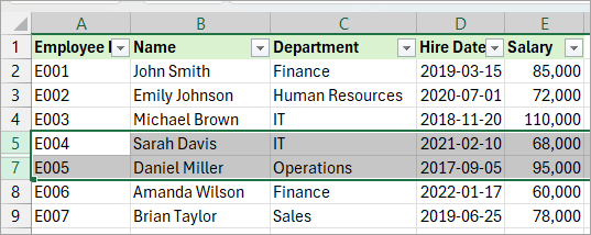
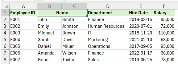
Reason #8: The Dataset Has Merged Cells in the Body
Cells C4 and C5 in the example dataset below are merged.
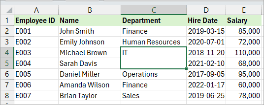
When you enable filtering and apply a filter for IT in column C, you get only one record instead of the two expected.
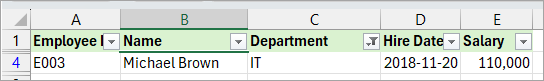
This happens because, in a merged range, Excel recognizes only the leftmost cell as holding the actual value. Excel considers all other cells in the merged range to be empty, even though the value appears to span two rows visually.
Fix: Unmerge the Cells
- Press CTRL+ SHIFT+L to clear the filter.
- Select the merged cells.
- Click the Home tab.
- On the Alignment group, open the Merge & Center drop-down and choose Unmerge Cells.
The above step unmerges the merged cells.
Enter separate values in the unmerged cells.
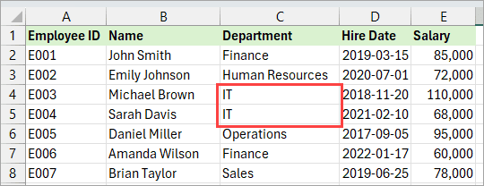
- Press CTRL+SHIFT+L to reapply the filter.
Reason #9: The Worksheet is Protected
When a worksheet is protected, the filter buttons on its data range become nonresponsive.
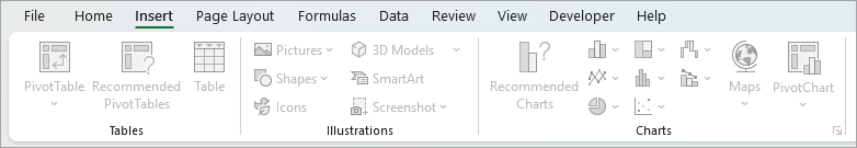
You can tell a worksheet is protected if many of the options on the Insert tab are disabled.
Fix: Unprotect the Worksheet
You can unprotect the worksheet using the steps below:
- Click the Review tab.
- Click the ‘Unprotect Sheet’ command button on the Protect group.
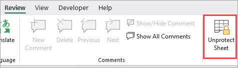
The above step opens the Unprotect Sheet dialog box.
- Enter the necessary password (if applicable).
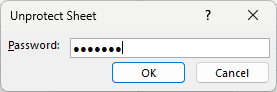
- Click OK.
Once the worksheet is unprotected, the filter buttons become responsive.
Reason #10: The Worksheet is Grouped
When a worksheet is grouped, the filter buttons on its data range become nonresponsive.
The clearest sign that a worksheet is grouped is the presence of [Group] next to the filename in the Excel title bar.

Another clue is that its sheet tab, along with one or more others, appears highlighted in white.

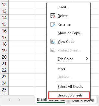
Fix: Ungroup the Worksheet
You can ungroup the worksheet using one of the three ways below:
- If all the sheets in the worksheet are grouped, click one worksheet tab at the bottom of the workbook to ungroup all the sheets.
- If only a few of the worksheets are grouped, click the worksheet tab of one of the ungrouped sheets to ungroup all grouped sheets.
- Right-click the tab of any of the grouped sheets and select ‘Ungroup Sheets’ on the shortcut menu.
Reason #11: The Worksheet is Corrupted
A corrupted worksheet can cause the Excel filter to malfunction.
Fix: Transfer Data to New Worksheet
Copy the data to a new worksheet. If the issue persists, reinstall Office.
I hope you found the tutorial helpful.
Other Excel articles you may also like: