EDATE Function in Excel

If you want to add or subtract a specific number of months from a date in Excel and land on the same day of the next month, the EDATE function is what you need.

In this article, I’ll walk through how EDATE works with practical examples, including per-row variable shifts, generating a monthly date series, and the end-of-month quirk that trips most people up.

⚠️ One thing to flag up front: EDATE is a legacy function from the old Analysis ToolPak, so it does not natively spill in Excel 365. The reliable pattern is per-cell with a copy-down. There is an array-coercion trick to make it spill across a column with a single formula, and I cover that toward the end.

EDATE Syntax

Here is the syntax of the EDATE function:

=EDATE(start_date, months)

• start_date – The starting date. A real Excel date, either a cell reference, a date created with the DATE function, or the result of another formula that returns a date.
• months – The number of months you want to add or subtract. Positive numbers go forward, negative numbers go backward. Decimals are truncated, not rounded.

When to Use EDATE

Use this function when you need to:

• Shift a date forward or backward by a fixed number of months
• Calculate per-row renewal, expiry, or follow-up dates where each row has its own months value
• Generate an evenly-spaced monthly series from a single start date
• Land on a day-aware date (e.g. the 15th of the next month, not just month-end)
• Calculate age milestones or maturity dates

Let me show you a few practical examples of how to use EDATE.

Example 1: Add Months to a Date

Let’s start with a simple example.

Below is a gardener’s planting log with seed-start dates in column A. I want a column of expected harvest dates 3 months later.

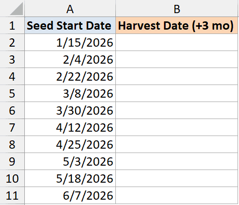
Here is the formula:

=EDATE(A2, 3)

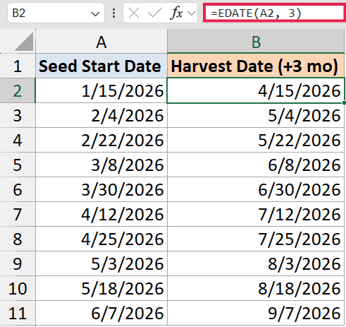
Enter this in B2 and copy it down. The 3 tells EDATE to step forward 3 months from each start date. So a start date of 15-Apr-2026 returns 15-Jul-2026.

If your result shows up as a number like 45913 instead of a date, format the cell as Short Date.

This is a much cleaner approach than adding months to a date by hand or piecing it together with DATE, YEAR, and MONTH.

Example 2: Subtract Months from a Date

Here’s the mirror version.

A museum has a list of exhibit closing dates in column A and wants a preview-event date that is 1 month before each closing.

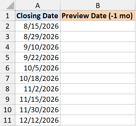
I want a preview date one month before each closing date.

Here is the formula:

=EDATE(A2,-1)

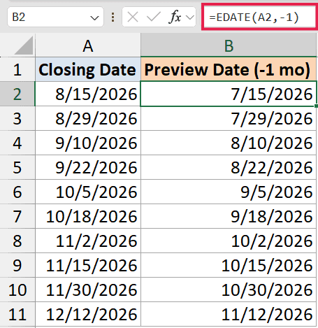
The minus sign tells EDATE to step backward. So a closing date of 15-Aug-2026 returns 15-Jul-2026. Copy this down the column for every row.

The same pattern works for any negative value. Pass -12 to land a year earlier, -24 for two years, and so on.

Example 3: Per-Row Variable Months (Subscriptions)

Now let’s look at something more interesting.

A magazine publisher has subscriber start dates in column B and the subscription length in months in column C.

The two columns vary per row, and you want a column showing each subscriber’s renewal date.

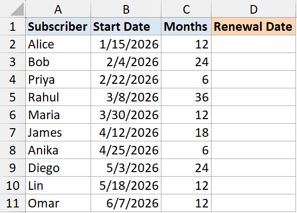
I want a renewal date for each subscriber, based on their own start date and length.

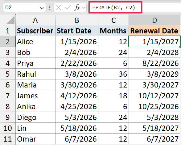
Here is the formula:

=EDATE(B2, C2)

How this formula works:

• A2 is the start date for that row.
• B2 is the subscription length in months for that same row. Some are 6, some are 12, some are 24.
• EDATE pairs each start date with its row’s months value and returns the renewal date.

Copy this down the column. If your data is in years instead of months, multiply by 12 inside the formula: =EDATE(A2, B2*12).

Pro Tip: For a running countdown to renewal, subtract TODAY() from the result. =EDATE(A2, B2)-TODAY() returns the days remaining for that subscriber.

Example 4: Generate a Monthly Series From One Start Date

Now let’s look at something a bit different.

You have a single date in A2 and you want a 12-month series of follow-up dates spaced one month apart, like a vaccine booster schedule or a

recurring billing calendar.

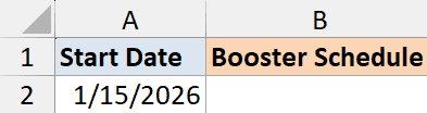
I want 12 dates, each one month after the previous, starting from the date in A2.

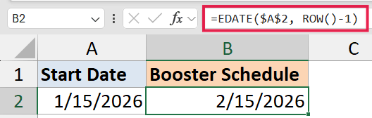
Here is the formula (enter in B2 and copy down to B13, or use the spill version below):

=EDATE($A$2, ROW()-1)

How this formula works:

• $A$2 locks the start date so it stays the same in every row.
• ROW()-1 returns 1 in B2, 2 in B3, 3 in B4, and so on. That’s the months offset for each row.
• EDATE shifts the start date forward by that many months, giving you a 12-row monthly series.

If you want to start at month 0 (so the first row is the original date), change the offset to ROW()-2. For quarterly instead of monthly, multiply the offset by 3: =EDATE($A$2, (ROW()-1)*3).

For a true single-formula spill version that doesn’t require copying down, see Example 6 below.

Example 5: End-of-Month Behavior (the Gotcha)

EDATE returns the same day-of-month in the result. So what happens when the start date is on the 31st and the target month doesn’t have a 31st?

Below is a pharmacy refill log where some prescriptions were started on month-end dates. Run EDATE to find the next month’s refill date.

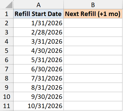
I want the next month’s refill date for each prescription.

Here is the formula:

=EDATE(A2, 1)

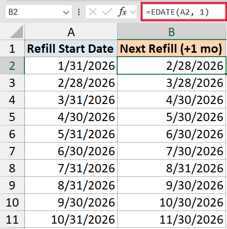
Run on 31-Jan-2026 and EDATE returns 28-Feb-2026, not 03-Mar-2026. The day clamps down to the last valid day of the target month. The same goes for 30-May-2026 → 30-Jun-2026 (no clamp needed), but 31-May-2026 → 30-Jun-2026 (clamp).

That clamping is usually what you want for monthly billing or refill cycles. But if your rule is “always land on the last day of the next month, no matter what day the start was on”, EDATE is the wrong tool. Use EOMONTH instead. =EOMONTH(A2, 1) returns the last day of the next month, regardless of whether the start was the 1st, the 15th, or the 31st.

EDATE matches the day. EOMONTH always snaps to month-end. Pick based on what your rule actually is.

Example 6: Spill EDATE Across a Range (the + Trick)

If you’re on Excel 365 and you’d rather write one formula than copy EDATE down a column, there’s a workaround.

EDATE is a legacy function from the old Analysis ToolPak, so it doesn’t natively spill the way modern functions do.

If you write =EDATE(A2:A11,3), you’ll get just one result, not an array. The fix is to add + at the beginning of the range to coerce the range into an array first that spills.

Below is a dataset where I want to spill the result of EDATE

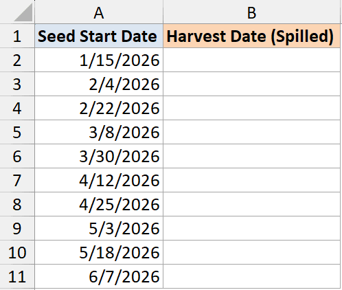
=EDATE(+A2:A11, 3)

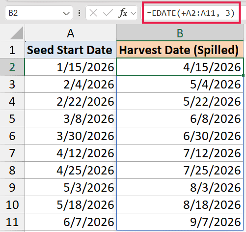
The + doesn’t change the dates themselves, but it forces Excel to evaluate A2:A11 in array context.

Once it’s an array, EDATE happily processes one date at a time and spills the results down the column.

The same trick works for other legacy date functions: EOMONTH, WEEKNUM, WORKDAY, NETWORKDAYS.

Tips & Common Mistakes

• EDATE does not spill on its own. Write =EDATE(A2, 3) and copy down, or use the +0 trick from Example 6 (=EDATE(A2:A11+0, 3)) if you want a single spilling formula.
• Result shows as a number – If EDATE returns something like 45678, the cell is formatted as General. Change the cell format to Short Date or any date format.
• #VALUE! error from text dates – EDATE needs a real Excel date, not text that looks like one. If your start_date is a string like “2026-01-15” pulled from another system, wrap it in DATEVALUE: =EDATE(DATEVALUE(A2), 6).
• #NUM! error – The result date falls outside Excel’s valid range (before 1-Jan-1900 or after 31-Dec-9999). Common culprit is subtracting too many months from an already-old date.
• Don’t confuse EDATE with EOMONTH – EDATE keeps the same day-of-month. EOMONTH always returns the last day of the target month. Pick based on what you actually want.
• Months arg truncates, not rounds – =EDATE(A2, 3.7) is treated as =EDATE(A2, 3). If you need exact day-level accuracy, work in days, not fractional months.

That covers EDATE in modern Excel. The per-cell pattern works reliably, the SEQUENCE-with-+0 trick gives you a single spilling formula in 365, and the end-of-month clamp behavior is now well-defined. For pure month-end snapping, pair it with EOMONTH.

List of All Excel Functions